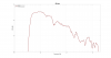
Here is the large test:
View attachment 67829
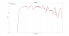
Here is my doing my best to match 11 of my scores to the results (discarding the lowest two):
View attachment 67832
The scores in the 5-6 range were a total guess as to which bubble it was, too clustered and no resolution.
EDIT: The 1.73 seems too large for that bubble, conforming it to ~20 PPO gives me 1.68. It looks to be around 1.55, I think it can be chalked up to slight errors in data extraction; and of course, which data points I deleted tp get to 20 PPO also is a factor.
Hi,
First I made a mistake on my PIR calculation.
Here is the correct formula:
Code:
PIR_calc1      = 10*log10( 0.12 * 10 .^ (Lwin/10) + ...
                           0.44 * 10 .^ (Erfx/10) + ...
                           0.44 * 10 .^ (Spow/10) ) ;
This gives IDENTICAL results to the NFS PIR.
I used the Ocean Way HR5 data from the NFS which I assumed is corrected for the PIR calculation (?).
In any case, even if the ER is not correctly calculated the formula for the PIR seems fine.
I just cannot understand the formula used by
@MZKM, could you explain it?
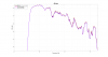
I am using the figure 10 of this paper which should (?) be the Olive metric for the 13 speakers of test one.
A Multiple Regression Model for Predicting Loudspeaker Preference Using Objective Measurements: Part II - Development of the Model
Here is the figure:
Here are the scores I scanned from it:
Data10a = [0.8486, 1.198, 1.223, 1.772, 1.6722, 2.5957, 3.6439, 3.7687, 4.0682, 4.792, 5.6406, 5.6406, 6.1398];
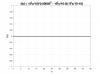
Here are the results with the corrected PIR for my calculation :
the difference between my calculation and
@MZKM could be explained by the PIR.
I am not expecting the data from the scanned Spinoramas to produce identical results but we should still be in the same ball park and we are obviously not.
Some points seem to be similar but we are not even sure if these scores correspond to the same speakers as I only rank the unlabelled score from low to high. What is more worrisome is the negative score.
IF all my assumptions are correct the score that we are calculating is not the Olive metric and therefore is of little merit.
@edechamps would you try the speaker #12 on the attached data (change .zip to . xlsx)
Edit:
I believe that the graph you used corresponds to this one in the original paper:
If we can get the similar score than that of the this graph:
EQ9:
Pref.Rating=6.04−0.67*AAD_ON−1.28*L
FX −0.66*LFQ + 4.02*SM_ON+ 3.58*SM_SP;
Scanned data:
data04 = [0.9141, 1.1514, 1.2888, 1.5144, 1.7349, 2.4452, 3.7617, 3.7781, 4.2299, 4.6261, 5.7719, 5.7995, 5.8983];
-> This gives access to SM_x and LFX
then
Get the same results for figure 13 a
the Equation are:
Pr
ef.
Rating = 2.63 −2.86*
NBD_
SP +5.15*
SM _
SP +0.417*
SL_
SP; EQ12
Scanned data:
data13 = [0.8232, 1.4264, 1.6589, 2.0359, 2.5889, 2.7208, 2.9596, 3.368, 3.8142, 4.9892, 5.0081, 5.737, 5.7873];
-> this gives access SM_x and NBD with SL_x easy to calculate (? invert the two lines from the table) :
Then we should be fine to calculate a more accurate score.
To me if SM is R2 both the manual and the direct Matlab calculation provide same results down to 13 decimals so it should be fine; "only", LFX, LFQ, NBD, AAD and SL need to be verified.
Cheers
M

 The only metrics that are common between the Test One and generalized formulas are LFX and SM.