Help with a math problem - converting Earthworks axial cal file to 90 deg

[jhaider]

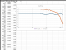
I'm trying to figure out a math problem that I thought would be easy but is ending up being more difficult than I expected. I'm trying to create a 90 deg cal file for an Earthworks M30. I have the current cal file ("ECF") as well as a "90 deg typical response" ECF from Earthworks. So I want to modify the mic's ECF to incorporate the HF compensation from the "typical response" file.

I've attached both files here.

PS: I realize I could crate a 90 deg cal file using John Reekie's method but I want to see if it can be done without introducing error from mic tip placement variation at HF in acoustic measurements.

 

[sam_adams]

This is the most important line from the article:

"One of the advantages of purchasing a microphone from Cross-Spectrum Labs is that you get a 90 degree calibration file included."

Send your mic to Herb and have him calibrate it. Then you have what you need—along with a reasonable measure of confidence that it's accurate.

 

[Blumlein 88]

Dayton Audio EMM-6 as good as UMIK-1 for someone who already has an audio interface?

That's not surprising. Even if the housing wasn't so similar, there are not that many mic companies who make their own capsules. That's true for any type of microphones. Two companies I know of that make high-end measurement capsules are Brüel & Kjaer and Microtech Gefell, and those are orders...

www.audiosciencereview.com

Here is a method to match two microphones using REW. You have the reference and create a second cal file for the second microphone. You could do the same thing comparing 0 degree with 90 degree. It is simpler than Reekie's method as you avoid having to dump it in a spreadsheet.

SIY had the idea of hanging a string with from the ceiling to position the microphone the same place twice. That would minimize the positioning error. Also I would position it more like a meter from a speaker. That also reduces differences in positioning somewhat. Still close enough reflections won't corrupt your measurement signals.

I would just use the typical file from Earthworks. The difference isn't really any response difference between mics. It is a difference in how the mic becomes directional. So the same difference applies to various EW mics, but will be consistent between 0 and 90 degrees as that is just physics.

 

[Blumlein 88]

I see EW didn't use the same frequencies for both files. That is rather bothersome. You could use it to get pretty close.

 

[NTK]

Is the math problem you are having due to the two files having different frequencies? If that is the case, then you just have to feed one of them into an interpolation function generator, and use it to interpolate numbers for the frequencies of the other. If you need more help, I should be able to come up with some python code for that in a day or two.

 

[jhaider]

This is the most important line from the article:

"One of the advantages of purchasing a microphone from Cross-Spectrum Labs is that you get a 90 degree calibration file included."

Send your mic to Herb and have him calibrate it. Then you have what you need—along with a reasonable measure of confidence that it's accurate.

I'm reasonably confident in Earthworks' calibration. Also note that the mic by itself is very good - tolerance band of 0.76 dB from 10-30k Hz if I can do math. So I realize I'm making this unduly difficult.

Is the math problem you are having due to the two files having different frequencies?

Sort of. But the basic math doesn't seem to be working out. What I tried to do was take the 10Hz

If that is the case, then you just have to feed one of them into an interpolation function generator, and use it to interpolate numbers for the frequencies of the other. If you need more help, I should be able to come up with some python code for that in a day or two.

"Interpolation function generator" is one of those things that I understand in concept but have no clue how to operationalize. But here I don't think it's a straight modification. The differences only manifest in the upper mids and beyond. So basically it's start with the specific mic ECF and carry that up to what looks to my eyes to be 2.2kHz, because that's where it looks like the mic starts to roll off when turned 90 deg. (Though that seems high to me - an iSEMcon EMX-7150's 0 and 90 deg cal files start to diverge at ~1250Hz, and that microphone has a slightly smaller tip than Earthworks M30.) Above that break point add rolloff function from the 90 deg generic file to the values in the unique ECF. The alternative approach might be to find a best fit function for the 90 deg file, and then adjust based on the variance in the ECF.

Here's an Excel screenshot showing the two files. Note the excessively exploded Y axis scale.

 

[Blumlein 88]

I believe you are over-thinking it. Just looking at your files I could match those that happen to be close and just do a straight-line interpolation between points. A straight line interpolation won't be exact, but it will always be in the right direction. There won't be any error more than .1 db at any point. Most points not even that much. That is good enough and then some in the real world use.

 

[NTK]

The attached text file contains the "90 degree typical data" resampled/interpolated to the frequencies in the "M30 on-axis calibration file". Below are the plots of the original data and results. The plot markers show the data points. The blue curve is the original 90 degree typical response, the orange curve is the M-30 mic specific on-axis response, and the green curve (offset by -4 dB) is the 90 degree response resampled to the frequencies of the M-30 data.

IMHO we'll also need the on-axis typical data, so we can calculate the delta between the on-axis and 90 degree data for the typical mic, and (assuming the delta is representative for all M-30 mics) apply the delta to the on-axis data of this specific mic.

Here is the Python code:

Spoiler: Python Code

# Read in 2 data files.
# Interpolate (resample) the first file (source data) to the x-coordinates as defined in the second file.
# Save the resampled data point pairs to a text file.
import numpy as np
from scipy.interpolate import pchip_interpolate

fname_in1 = '90_Degree_M_Series_Typical_Response.txt'
data_in = np.loadtxt(fname_in1, delimiter=',', skiprows=1)
fname_in2 = 'Earthworks M30 - on axis.txt'
interp_coord_target = np.loadtxt(fname_in2, delimiter=',', skiprows=2)

# Remove any target x-coordinates that are outside the range of x in the source data
x_interp = interp_coord_target[:, 0][np.logical_and(interp_coord_target[:, 0] > data_in[0, 0],
                                                    interp_coord_target[:, 0] < data_in[-1, 0])]
# Add the 2 end points of the source data if the target x-coordinates end points aren't near them.
if np.abs(x_interp[0] - data_in[0, 0]) > 0.5:
    x_interp = np.r_[data_in[0, 0], x_interp]
if np.abs(x_interp[-1] - data_in[-1, 0]) > 0.5:
    x_interp = np.r_[x_interp, data_in[-1, 0]]

# Use the PCHIP method for the interpolation.
# Since the x-coordinates in the data files are octave (i.e. log) spaced, it is better
#  numerically to interpolate using the logs of the x-coordinates as the data fed
#  into the interpolator will be more linearly spaced.
y_interp = pchip_interpolate(np.log10(data_in[:, 0]), data_in[:, 1], np.log10(x_interp))

# Save resampled data to the new x-coordinates to the format of the source data file.
fname_out = '90_Degree_Response_Interpolated.txt'
np.savetxt(fname_out, np.vstack((x_interp, y_interp)).T, fmt='%.3f',
           delimiter=',',  newline='\n', header='"Hz","dB"', comments='')

The interpolation method used is PCHIP (piecewise cubic Hermite interpolating polynomial). For an introduction to numerical interpolation, please see the chapter on Interpolation:

Numerical Computing with MATLAB

www.mathworks.com

 

[jhaider]

IMHO we'll also need the on-axis typical data, so we can calculate the delta between the on-axis and 90 degree data for the typical mic, and (assuming the delta is representative for all M-30 mics) apply the delta to the on-axis data of this specific mic.

Thanks for that! Empirically I agree with you. Intuitively though I would think that the 90 deg correction should be a pretty straightforward curve fit. The small lumps and bumps in the "typical" curve are likely properties of the DUT. Now that I have resampled data points maybe I'll play around with some curve fit functions in Excel and see if it makes sense.

(And yes, @Blumlein 88 - well, well aware that I'm overthinking.)

 

[jhaider]

Well...I took the interpolated "typical" data from @NTK, smoothed it by eyeball out under the assumption that the minor lumps and bumps in its curve were from the DUT (the "typical" curve zigs where my microphone zags in a couple regions). I normalized both to 0dB at ~1kHz, and spliced the sum of the ECF and smoothed interpolated curve to the ECF where they started to diverge to account for the divergence from flat (by tenths of a dB) in my microphone.

Results:
(Dark blue = 0 deg ECF; Red: NTK interpolation, normalized; Green: eyeballed "fix" for NTK interpolation; Light blue = synthetic 90 deg cal file)

Of course @Blumlein 88 is right that this is all a little silly. OCD is the only real reason to do this rather than just using the generic 90 deg file for this microphone. Here's the difference when plotted on normal scale.