Note: this is a slightly revised version of an article I wrote for the Widescreen Review Magazine. It was published in January 2014 I think.
-----
A Deep Dive into HDMI Audio Performance
Sometimes I feel that digital audio is the most misunderstood technology around. If I asked you how a TV works you likely will give me a blank stare. But if I ask how digital audio works I will immediately get answers. Unfortunately those answers are often not correct.
The misconceptions are caused by our familiarity with another digital technology: computers. We equate how things work there for how they work in the digital audio domain. For example, copying a file from a hard disk to a flash thumb drive produces an identical file. By the same token we think that digital audio also means perfect reproduction. Such is not the case. Just because it has the word “digital” in it doesn’t mean it works like it does inside our computers. The reference “digital” relates to the input of the system, not its output. At the risk of stating the obvious, the output is an analog signal – something entirely different than how our computers operate for us. Let’s review how it works.
Digital Audio Architecture
Figure 1 shows the basic block diagram of a Digital to Analog Converter (DAC). As we expect, there are digital samples on its input in the form of “PCM” formatted values. The DAC is either part of a dedicated device by the same name, an Audio Video Receiver (AVR), or a Home Theater processor. The source of the digital stream is often separate device in the form of a Blu-ray player, cable, satellite or Internet set-top box or a computer acting as music or movie server. In these situations the digital data exists in the source and is transmitted over some sort of cable to the device that contains the DAC. The interconnect can be HDMI, S/PDIF (coax), Toslink (optical), network connection (wired or wireless) or a computer connection such as USB.
There is an unwritten rule about the design of consumer electronics equipment that says the source is the master. This means that the source determines the rate at which the downstream device, in this case the DAC inside your equipment, needs to output the digital audio samples. The simplest case is whether the data is 44.1 KHz sampling as is the case for CD music or 48 KHz as it is for most movie content. The source makes that determination based on what content it is being told to play (or manual “upsampling”) and the downstream device has to follow. If it does not, there can be problems such as losing audio and video synchronization.
All digital audio systems need a clock. This is a train of pulses that tell the DAC when to convert a digital audio value into an actual analog signal on its output. That clock could be “locally” produced meaning a circuit sitting right next to the DAC. Due to the above rule however, we cannot do that. Instead, we need to “listen” to the source and have it tell us how fast we need to play. This is done by monitoring the digital pulses on the incoming signal over say, HDMI or S/PDIF and determining the clock rate from that. In figure 1 you see this indicated by the “clock pulses” input.

Figure 1 Basic block diagram of a Digital to Audio Converter (DAC)
When you move the source of your timing upstream of a device the job of capturing that data becomes challenging. Cables are not perfect transmission lines and can distort the pulse stream. That distortion causes the receiver to guess incorrectly the precise rate of audio streams. When this happens, we introduce a special kind of distortion into the analog output of the DAC called “jitter.” Figure 2 shows how this occurs. By moving the time at which we change the output value, we deform the waveform and with it, create distortion.

Figure 2 Jitter timing distortion (courtesy, Prism Sound).
Figure 2 is the “time domain” representation of jitter distortion. We can transform that into frequency domain and get a better feel for what it means audibly. Unfortunately it is not so easy to make that determination because to do so we need to know how the jitter timing changed. Two cases of it are simple to analyze though:
If you go back to diagram 1 you see that there is another input to our DAC called the “voltage” reference. A DAC’s job is to output an analog voltage relative to a reference. Let’s say you set that reference to 1 volt and you feed the DAC 16 bit samples. The smallest number there is zero and the larger 65535. The DAC is expected to output distinctly different voltages as you increase the values from 0 all the way up to 65535. For the DAC to work perfectly, then it needs to add increments of 1/65535 or 0.00001526 volts for each increment in the input value. These are awfully small incremental voltage changes. Any instability in the reference voltage due to noise, or other frequencies riding on it, even if they are very small can create distortion on the output of the DAC.
Fortunately for us, DACs today (with rare exceptions) are built around dedicated parts with excellent performance. We are talking about signal to noise ratios of 120 dB which, if you recall my previous articles, is the performance target we aim at to arrive at transparency relative to the dynamic range of live music and the best we can achieve in our listening rooms. The DAC chip specs are “bench performance” meaning the device is tested in isolation. Put that same chip inside an AVR with a lot of other processing such as video and audio and all bets are off. Without careful engineering such as keeping the clock very clean and the reference voltage solid, performance can easily drop below the manufacturer specifications.
Note that we don’t even need a physical connection between the rest of the circuits and the DAC.I am sure you are familiar with the concept of receiving a radio transmission (RF) over the airwaves. Same here. RF signals are generated by electronic circuits and can bleed into the DAC.
Our main defense against all of this is the skill of the engineers who designed the DAC chip, and the device that contains it. High performance implementations can deliver precisely what we need. Alas, due to cost, size, skill and time to market limitations, equipment makers often miss the target. Worse yet, when that occurs we don’t get to know about it as there is a dearth of deep analysis for digital audio performance in the home theater market. The pure “2-channel” stereo market is served by magazines which perform detailed analysis of digital audio products. Those magazines however do not care about multi-channel systems so you don’t see reviews of AVRs and processors in them. HiFi News in the UK used to be an exception but they also stopped testing such products. So sitting here today, there is not a single published measurement of digital audio product for any AVR you may be thinking of purchasing! Yes, there are measurements of amplifier power and such, but nothing beyond that.
Even when digital measurements exist, they are next to impossible for the average enthusiast to understand. This is partially due to unfamiliarity with the architecture of the system which hopefully is now remedied per my earlier explanation, due the very non-intuitive way we test digital systems. So let’s get that problem out of the way too.
Digital Audio Measurements
The goal we have here is to tease out the distortions from the system. Traditional measurements such as frequency response are boring as DACs have nearly ruler flat response. Instead, we want to search for data that tells us the problems I described earlier are occurring and with it, causing us to miss our dynamic range we need to achieve transparency.
If you look at digital audio measurements, you usually run into a test signal called “J-Test.” J stands for jitter. J-Test was created by the late Julian Dunn when he worked for Prism Sound. It was designed to find cable related jitter in both professional (“AES”) and consumer (S/PDIF) digital audio transmission lines. How this is accomplished is beyond the scope of this article but what you need to know is that J-test is a combination of two square waves. One is a near full amplitude one and the other, at the smallest one we can represent. The frequencies of these are proportional to the sampling rate of audio. For 48 KHz, which is the signal I used for this test, the large square wave runs at 12 KHz and the small one, at 250 Hz. If you feed this signal to a perfect DAC, what comes out of it is a sine wave. Yes, you heard me right. What comes out is a sine wave. How does a square wave become a sine wave?
There are two reasons for that. The first is that digital audio sampling theory says that system bandwidth must be limited to half of its sampling rate. A 48 KHz sampling system must therefore have no more bandwidth than 24 KHz. When we first digitize analog signals, we filter anything past 24 KHz and likewise, we must limit the analog output of the DAC to 24 KHz. The other concept we need to understand is that a square wave can be decomposed into an infinite series of sine waves. The first one is at the same frequency of the square wave and the rest, odd-integer harmonics (multiples) of that. Figure 3 shows an example for a 1000 Hz square wave. Notice how the multiples are at 3000, 5000, 7000 Hz and so on.

Figure 3 Square wave spectrum.
Please stay with me, we are almost there! If we feed the J-test square wave to our DAC, it will filter frequencies above 24 KHz. Since our harmonics in our square wave start at three times 12 KHz or 36 KHz they will be gone due to this filtering, leaving us with just the original 12 KHz which now is a sine wave. This fact becomes important later when I show the full spectrum of the DAC output including frequencies above 24 KHz. We get to see that DAC filters are not perfect and will let through some of those harmonics.
In this article I will be analyzing the performance of HDMI, a digital transport which carries both audio and video over the same cable. The audio is embedded in the unused portion of the video. Since audio bandwidth is much lower than video, the spare area for video was deemed sufficient to put it there. Alas, this means that you cannot have audio without video. Let me repeat: with HDMI you must carry video in order to receive audio as that latter data is fit into the actual scan lines of video. You will see later how this can cause performance problems for us. For now, I want to note that the J-Test signal is not able to do what it does in S/PDIF. Namely, it is not able to cause any distortion to become visible due to cable effects.
Now that you are smarter than all of your friends about principals of digital audio, let’s get into the meat of this article which is measuring some of the devices we may own.
Measurement Setup
For this article, I had a special interest in contrasting the performance of S/PDIF against HDMI. S/PDIF as you may know, was introduced by Sony and Philips (S/P in that name) when the CD format was first developed. So we are looking at a standard that is about 30 years old now. Over those years, a lot has happened to optimize its performance despite some design mistakes in how it works which help induce jitter. HDMI in contrast is a much newer standard with the first implementation dating back to 2003. Still, we are talking about a solution that has been out nearly a decade so one would expect it to be at a refined stage. We set out to test this theory.
To measure small distortions we need the right instrument. When I started on this project my plan was to use my Audio Precision (AP) analyzer. While the AP is a capable device with sufficient resolution to show us distortion products in our DACs, it leaves something to be desired from a usability point of view. It is a stand-alone product designed mainly to generate its own test signals. In my case, I wanted to use a PC as the source since I can quickly change from one output format (HDMI) to another (S/PDIF). This made it very challenging to use the AP as I would then need to replicate its signals on the PC and manually run them.
A fortuitous thing occurred while I was walking the CES show where I ran into the good folks at Prism Sound. You may not have heard of Prism Sound but they produce some of the finest professional analog to digital (ADC) and digital to analog converters (DAC) for the professional market. Out of necessity, they designed their own test instruments. The latest generation is the dScope III series of analyzers. These are basically super high performance DACs and ADCs with PC software that turn into purpose built analyzers for testing of digital and analog products. The key differentiation in my case was that the system is able to use the PC for signal generation just as it is able to generate signals itself. This would have made my testing much simpler. So imagine my delight when I asked if I could borrow their equipment to use for this project and hearing them immediately say yes!
A bit more about the test fixture: the source is my Vaio Z series laptop. This has an nVidia GPU (graphics processor) which outputs HDMI. The machine also has two USB ports. I used one to communicate to the dScope analyzer. And the other was connected to a USB to S/PDIF converter. The unit of choice there was the Berkeley Audio Design Alpha USB. This is a very high performance USB to S/PDIF converter which looks acts like a sound card for your PC or Mac. It takes data over USB and outputs an isolated and super clean S/PDIF signal with minimum jitter and noise. Its operation is in “asynchronous” mode which I will outline in a future article. For now, take my word for it that this mode of operation is the key to keeping the PC from adding its own jitter to the S/PDIF connection.

Figure 4 Test fixture comprising of a Sony Z-series laptop with HDMI output. S/PDIF was generated using a Berkeley Audio Designs Alpha USB. Output drove the device under test (AVR, DAC or processor), the analog output of which was analyzed by the Prism Sound dScope analyzer.
I used Windows 7 as my OS. dScope software uses the standard Windows audio “stack” (code) to talk to HDMI audio and USB to S/PDIF. The Windows audio stack converts audio samples to a high resolution (floating point) internal format. On the way out to the sound device this is converted back to integer PCM samples. To eliminate distortion that this conversion can create, it adds “dither” (noise) to the PCM samples. It also converts all audio samples to a fixed sample rate. To use a PC as an instrument, or frankly as a high-performance audio server, it is critical that these settings be appropriately configured. Since all of my testing was at 48 KHz, I changed the advanced properties for both HDMI audio and Berkeley to be the same as that. The default is 44.1 KHz which invokes the kernel resampler causing some distortion products. To reduce the impact of dither noise, I set the output format to 24 bits. Since dither impacts the lowest bits in our samples, and no device is cable of doing much better than 20 bits of resolution anyway, selection of 24 bits essentially eliminates the effect of Windows audio stack dither. The default is 16 bit output which will definitely show up as elevated noise floor.
Now, even though jitter is a timing clock problem, we don’t measure its effects at the clock input of the DAC. The reason is that we can’t access that part easily anyway and at any rate, the DAC is supposed to have circuits in it (called PLL) that help to reduce its rate (in theory anyway; see later section in this article). Best then is to sample the analog output of the DAC, just like how we would listen to it normally, and see what distortion we have there. Ditto for any other type of distortion. For AVRs, I used their pre-amp outputs. For DACs and processors, I naturally used their analog outputs. I used unbalanced (RCA) in all cases even if the device had balanced (XLR) output.
So the setup from end to end involves selecting HDMI or USB/S/PDIF output, running J-Test into the DAC, setting the levels close to or at max, and then performing the measurements. On levels, I made it all relative so that we can compare device to device (DACs can have different amplitude outputs). The standard in the industry is to use the “dbFS” scale. dB means decibels. FS means relative to full scale. 0 dbFS is the maximum signal and is the level I set for every DAC under test. Therefore all values are negative relative to that. Since these are noise or distortion levels we are talking about, the lower or more negative the number, the better.
Not being a professional reviewer, I had to come up with all the equipment to test on my own. I first drew on my stock of older equipment I keep around. I then went rummaging through our demo inventory at work (Madrona Digital). The result is an odd mix of new and old gear which should provide good comparison between classes of products and advancement in technology (or lack thereof as you see). Here is the full list:

Figure 5 Test equipment and devices tested.
The Measurement Results
Let’s start with the best of the best so that we get calibrated on what good results look like. Remember, the source signal was J-Test and the outputs are in frequency domain. If all goes well, we should see a single tall spike representing the 12 KHz signal and nothing but noise at very low levels. Here is a picture perfect measurement from the Mark Levinson No 360S DAC:

Figure 6 Mark Levinson No 360 S
There are two symmetrical spikes which likely are jitter induced (I did not have time to isolate the cause as jitter or voltage modulation). Their levels are completely benign at -123 db. For grins, let’s go past the DAC’s 24 KHz response and our hearing range to see what is going on in the ultrasonic area:

We see a set of harmonics of our 12 KHz test tone at 24 KHz, 36 KHz and so on. None is a cause for concern since we don’t hear much spectrum above 20 KHz, and even if we could, we would not have much of a prayer to perceive them at such low levels (roughly -90 dBFS worst case).
Now let’s look at a mass market AVR from our list using HDMI:

Now that is a big difference if there ever was one. Let’s see if we can explain some of it. First we notice the rising noise level in both ultrasonic and low frequencies. This is called “noise shaping” and is a tactic in DAC design to push the noise out of the middle frequencies where our ears are most sensitive into an audio spectrum that is not as audible (anything above 20 KHz is definitely fair game). Without this technique, the noise floor would have been higher in the middle frequencies. Beyond the noise shaping, there are also a number of distortion spikes but since we are zoomed out too far, they are hard to distinguish. So let’s focus back on the 0 to 24 KHz and add to it the S/PDIF performance (in blue):

We can see that our noise floor is -110 to -115 dB which is 10 to 15 dBs higher relative to the Mark Levinson. Importantly, we have a lot of new distortion products, especially in HDMI. Let’s zoom in some more to see them better:

Oh boy! Look at those symmetrical spikes in red when we use HDMI. Their levels are close to – 90 dB which is quite a bit higher than the worst ones for S/PDIF. Clearly we have taken a step backward with HDMI. Remember, this is the exact same DAC being driven inside the AVR. The only difference is which “digital” connection we used to drive it. Clearly “digital is not digital” as these two measurements show. Changing the digital connections upstream changed the analog output of the DAC downstream.
Note that beside the distinct distortion products, there is also the broadening of the shoulders in our main pulse at 12 KHz. In blue with S/PDIF we have a narrow spike as we should. But with HDMI in red, it widens to about 600 Hz on each side. This is band limited noise that is likely polluting the DAC clock.
This paints a pretty bad picture for HDMI. What is going on? Is HDMI flawed itself? Let’s look at the Mark Levinson 502 for more clues. Here is its HDMI measurement (in yellow) compared to the above AVR (in red). Note that the vertical scale is -80 dB so we are zoomed in like the above display:

Comforting is the fact that that the Mark Levinson maintains its composure by producing excellent noise floor hovering in -125 to -130 dbFS. We also have much less noise around our main signal which is nice to see. No device came remotely close to the performance of the Mark Levinson in HDMI.
That said, HDMI did leave its thumbprint on the device. We see a few distortion spikes that interestingly enough line up with the exact same ones in the above AVR. The common theme between these two measurements is my laptop and HDMI and therefore the arrows directly point to them. Let’s see if we can narrow this down some. Let’s test S/PDIF performance this time with and without the HDMI cable plugged in:

First we notice the wonderful performance of this processor with S/PDIF without the HDMI connection in teal color. Again, the Mark Levinson beats all other home theater products and is only bested by its older sister, the No 360 S DAC.
What is newsworthy is the appearance of the amber spikes which only appeared when I plugged in the HDMI cable while still measuring S/PDIF. We see a spike showing up at 7,163 Hz with a level of -114 dBFS. This same distortion spike was present when we tested HDMI as the input. This means that this kind of spike is not related to how HDMI works per se but the fact that the mere use of it causes noise to be induced from the source into the target device. Let me repeat: the mere act of connecting an HDMI cable to your DAC causes its performance to decline!
As I mentioned, the Mark Levinson outperformed all the other devices over HDMI. Here is a comparison shot demonstrating that:

The Mark Levinson 502 is in gray at the bottom. No other device is able to match its low noise floor. Remember that every 3 dB difference here means doubling of the amplitude of the noise or distortion. So differences of 10 to 20 dB are actually quite large and require a lot more careful design to achieve. Considering that some of these devices are much newer, it sadly points to a picture of technology not improving with time.
Here is an enlarged version of the above graph centered around the 12 KHz J-test signal:

There are distinct performance levels here with identical HDMI input signal.
The Hits Keep Coming
Take a look at these two measurements:

Would you believe this is the exact same device being measured consecutively with absolutely no change in the setup? As I measured over and over again, the output would ping pong between these two types although not predictably. The additional noise and distortions are likely due to varying activity in the rest of the system. Even with other devices that had more stable operation, run to run variations were observed.
Let’s see if we can make ourselves feel good by looking at more S/PDIF measurements:

The yellow is the Lexicon 12B and the red, the Tact RCS 2.0. We see the family resemblance in the Lexicon to its sister companies (Harman owns Mark Levinson and Lexicon): smooth and clean noise floor below -120 dbFS. None of the drama of HDMI exists here.
The Tact performance is odd though. It has generally lower noise floor but then has a bunch of spikes around the main signal. The psychoacoustics principal of masking says that these distortions are too close to the mains signal to be audible. So perhaps this is a good choice. If it were up to me though, I would aim for the Lexicon performance.
Here is another hopefully interesting comparison, this time testing the Peachtree decco65 with its USB input vs. S/PDIF fed by the Berkeley adapter:

We see the Berkeley results are cleaner. Remember again that throughout these tests we are always testing digital interfaces. Here we are testing two ways of outputting audio over USB. One is with a dedicated device in the form of Berkeley and another with the interface built into the DAC. The comparison could be a lot more lopsided than this as the decco uses the same advanced “asynchronous” USB.
The pulses look a bit too regular to be noise. So let’s zoom in to see what is there:

The curser is at “58.59” Hz which, if we account for some slight measurement error, we can conclude it is really at 60 Hz or the line frequency of our power supplies in US. The 60 Hz cycle repeats throughout the entire spectrum with the Berkeley interface showing less of that. It is unfortunate that the power supply was not as isolated as it could have been. Still, all in all, this device performs quite well relative to the mass market devices.
Let’s compare the S/PDIF performance of a few devices at once:

The red curve at the bottom is what we started with: the Mark Levinson No 360S DAC. It seems that 13 years later we still can’t do better. Above the Mark Levinson in teal is the decco using the Berkeley as its interface. Above it is the two AVRs. You get the picture.
Good Design, Bad Design
While on the subject of S/PDIF, let’s run another fun test. Remember what I said at the start of this article: our sources are the master. They generate the clock timing that the receiver must follow. While we want the receiver to follow the source, we only want it to do so with respect to generally playing the right number of samples per second. Ideally, it would not chase the errors induced by the cable or noise/distortion variations in the source. DACs implement a clock extraction/generation circuit called PLL. The PLL can be designed to filter out these variations. There are industry recommendations for both professional and consumer digital audio connections to do exactly that. It calls for a lot of filtering at higher frequencies (where it is easier) and reasonable amount at lower frequencies.

For grins, I decided to test the performance of a handful of devices to see how well they do in this respect. For this testing I used the Audio Precision Analyzer as the source since it is able to inject jitter at a specific frequency. By sweeping the jitter frequency from high to low and measuring the output of the DAC, we can determine if the above guideline is implemented. Here is what we get:

Starting from the bottom and going up, we have the Mark Levinson No 360S DAC in yellow, the Mark Levinson No 502 Processor in pink, then the Lexicon 12B in brown, and then a bunch of AVRs clustered around the zero line. Remember this is a log scale. So 60 dB means 1,000,000 times more attenuation than 0 dB. That is what the Mark Levinson DAC achieved. The Mark Levinson and Lexicon processors also did an excellent to good job of reducing jitter respectively.
Unfortunately the AVRs just sat there and took it all in. Not good. Not good at all. Translating, even when it comes to S/PDIF we are finding sloppy engineering in mass market devices. You better use very clean sources like I did with the Berkeley USB adapter. That device has an ultra-clean clock source and high isolation from the PC and therefore has much less reliance on the target device to clean up its signal. If you have an AVR, using a high quality asynchronous USB to S/PDIF adapter may be one of the best “tweaks” you can use to improve its performance (for music applications).
A Note on Audibility
I have shown you a lot of graphs but it would be unfair to leave them be as is. A lot of the distortions we see with HDMI are centered close to our main excitation frequency. When the distortions are close to a loud signal, and our source certainly is one in this case, they can’t be heard. So mostly like these are not audible distortions. As we get farther from the main tones, the spikes can reach higher than level of audibility and the chance of this occurring with HDMI is higher than with S/PDIF.
Summary and Final Thoughts
Digital audio is a complex area of audio. Characterizing its performance requires a good understanding of how it works, going beyond common misconceptions of it being “bit perfect.” The measurements show that HDMI is a setback from a performance point of view. While “heroic” efforts such as the Mark Levinson 502 manage to get superlative performance out of HDMI, it clearly presents a tough situation for lesser designs. More concerning is that the mere connection of a device to an HDMI source can cause it to degrade its performance over other inputs. Other anomalies include performance that is dynamic in ways that is not common in consumer electronic products.
Stand-alone dedicated devices such as the Mark Levinson DAC, the Peachtree decco65, and the Berkeley Audio Design Alpha USB interface show that when engineers focus on producing better quality they indeed get there, albeit at premium prices.
Sadly we did not find evidence of time making things better. Older products such as the aforementioned Mark Levinsons and Lexicon ran circles from a measurement point of view around the newer devices. Clearly this is another example of digital audio not following other digital technologies such as computers.
My advice is that if you are using your system for critical music listening, use S/PDIF instead of HDMI. If you are using a PC or Mac as the source, invest in a high-quality USB to S/PDIF converter.
As you may have noticed, I have not disclosed the identity of the systems that did not perform well here. My hope is that these companies take notice and improve their designs. It used to cost a lot for such instrumentation and hence the testing that I performed. In today’s dollars, my Audio Precision would set you back $30,000+. But innovations like the Prism Sound dScope have changed this landscape considerably. The version I used costs $9,895 which should be next to nothing for companies developing consumer electronics for mass markets. Some careful attention to circuit design and a few more dollars in parts should get us better performance. Let’s hope the next time I test these products, we see much better results.
Note 1: The references to absolute noise floor in this article (e.g. 120 dbFS) are not strictly correct in that the noise floor is partly determined by the characteristics of the measurement (i.e. FFT process gain). So it is best to use these measurements to compare products to each other as they all use identical parameters used for each.
I would like to sincerely thank the team including Simon Woollard,Ian Heaton,Graham Boswell, and Doug Ordon at Prism Sound for the kind loan of the dScope III, and their helpful advice, without which this article would not have been possible. Additional thanks for their kind permission to use some of the graphics from their presentation.
References
"Performance Challenges in Audio Converter Design," Ian Dennis, Prism Sound Systems, AES 24th UK CONFERENCE 2011
“The Diagnostic and Solution of Jitter-related Problems in Digital Systems,” Julian Dunn and Ian Dennis, Prism Sound Systems, AES 96th Convention, 1994
“Considerations for Interfacing Digital Audio Equipment to the Standards AES-3, AES-5, AES-11,” Julian Dunn, Prism Sound, 10th International Conference: Images of Audio (September 1991)
“The Numerically-Identical CD Mystery-A Study in Perception Versus Measurement,” Lan Dennis, Julian Dunn, and Doug Carson, AES Conference: UK 12th Conference: The Measure of Audio (MOA) (April 1997)
“Audio Engineering and Psychoacoustics: Matching Signals to the Final Receiver, the Human Auditory System,” Eberhard Zwicker and U. Tilmann Zwicker, JAES Volume 39 Issue 3 pp. 115-126; March 1991
Amir Majidimehr is the founder of Madrona Digital (www.madronadigital.com) which specializes in custom home electronics. He started Madrona after he left Microsoft where he was the Vice President in charge of the division developing audio/video technologies. With more than 30 years in the technology industry, he brings a fresh perspective to the world of home electronics.
-----
A Deep Dive into HDMI Audio Performance
Sometimes I feel that digital audio is the most misunderstood technology around. If I asked you how a TV works you likely will give me a blank stare. But if I ask how digital audio works I will immediately get answers. Unfortunately those answers are often not correct.
The misconceptions are caused by our familiarity with another digital technology: computers. We equate how things work there for how they work in the digital audio domain. For example, copying a file from a hard disk to a flash thumb drive produces an identical file. By the same token we think that digital audio also means perfect reproduction. Such is not the case. Just because it has the word “digital” in it doesn’t mean it works like it does inside our computers. The reference “digital” relates to the input of the system, not its output. At the risk of stating the obvious, the output is an analog signal – something entirely different than how our computers operate for us. Let’s review how it works.
Digital Audio Architecture
Figure 1 shows the basic block diagram of a Digital to Analog Converter (DAC). As we expect, there are digital samples on its input in the form of “PCM” formatted values. The DAC is either part of a dedicated device by the same name, an Audio Video Receiver (AVR), or a Home Theater processor. The source of the digital stream is often separate device in the form of a Blu-ray player, cable, satellite or Internet set-top box or a computer acting as music or movie server. In these situations the digital data exists in the source and is transmitted over some sort of cable to the device that contains the DAC. The interconnect can be HDMI, S/PDIF (coax), Toslink (optical), network connection (wired or wireless) or a computer connection such as USB.
There is an unwritten rule about the design of consumer electronics equipment that says the source is the master. This means that the source determines the rate at which the downstream device, in this case the DAC inside your equipment, needs to output the digital audio samples. The simplest case is whether the data is 44.1 KHz sampling as is the case for CD music or 48 KHz as it is for most movie content. The source makes that determination based on what content it is being told to play (or manual “upsampling”) and the downstream device has to follow. If it does not, there can be problems such as losing audio and video synchronization.
All digital audio systems need a clock. This is a train of pulses that tell the DAC when to convert a digital audio value into an actual analog signal on its output. That clock could be “locally” produced meaning a circuit sitting right next to the DAC. Due to the above rule however, we cannot do that. Instead, we need to “listen” to the source and have it tell us how fast we need to play. This is done by monitoring the digital pulses on the incoming signal over say, HDMI or S/PDIF and determining the clock rate from that. In figure 1 you see this indicated by the “clock pulses” input.
Figure 1 Basic block diagram of a Digital to Audio Converter (DAC)
When you move the source of your timing upstream of a device the job of capturing that data becomes challenging. Cables are not perfect transmission lines and can distort the pulse stream. That distortion causes the receiver to guess incorrectly the precise rate of audio streams. When this happens, we introduce a special kind of distortion into the analog output of the DAC called “jitter.” Figure 2 shows how this occurs. By moving the time at which we change the output value, we deform the waveform and with it, create distortion.
Figure 2 Jitter timing distortion (courtesy, Prism Sound).
Figure 2 is the “time domain” representation of jitter distortion. We can transform that into frequency domain and get a better feel for what it means audibly. Unfortunately it is not so easy to make that determination because to do so we need to know how the jitter timing changed. Two cases of it are simple to analyze though:
- The change is sinusoidal, i.e. the timing changes themselves follow a sine wave. When this occurs, we get two distortion products that are proportional to the jitter amplitude (i.e. how much we move the audio samples in time). If we have a 12 KHz tone and we apply a 2 KHz sinusoidal jitter to it, we get new “side band” distortions at 10 KHz and 14 KHz. If jitter were at 3 KHz, then the side bands would be at 9 KHz and 15 KHz and so on.
Our analog systems such as amplifiers usually create what is called harmonic distortion. If we had the same 12 KHz signal, the harmonic distortion would be at 24, 36, 48 KHz and so on. This is very different than our jitter distortion where there is no harmonic relationship. Such non-harmonic sounds do not appear in nature and hence, we tend to notice them more often.
- The change is random, i.e. noise like. When we change the timing of each output sample randomly, then what we create is noise on the output of the card. The reason is that noise is a rich spectrum of primary tones. Therefore what we are doing is applying jitter at countless frequencies to our source so we get countless distortion products. Clustered together, they no longer look like individual distortion spikes but an infinite number of them and hence, will be perceived as noise.
If you go back to diagram 1 you see that there is another input to our DAC called the “voltage” reference. A DAC’s job is to output an analog voltage relative to a reference. Let’s say you set that reference to 1 volt and you feed the DAC 16 bit samples. The smallest number there is zero and the larger 65535. The DAC is expected to output distinctly different voltages as you increase the values from 0 all the way up to 65535. For the DAC to work perfectly, then it needs to add increments of 1/65535 or 0.00001526 volts for each increment in the input value. These are awfully small incremental voltage changes. Any instability in the reference voltage due to noise, or other frequencies riding on it, even if they are very small can create distortion on the output of the DAC.
Fortunately for us, DACs today (with rare exceptions) are built around dedicated parts with excellent performance. We are talking about signal to noise ratios of 120 dB which, if you recall my previous articles, is the performance target we aim at to arrive at transparency relative to the dynamic range of live music and the best we can achieve in our listening rooms. The DAC chip specs are “bench performance” meaning the device is tested in isolation. Put that same chip inside an AVR with a lot of other processing such as video and audio and all bets are off. Without careful engineering such as keeping the clock very clean and the reference voltage solid, performance can easily drop below the manufacturer specifications.
Note that we don’t even need a physical connection between the rest of the circuits and the DAC.I am sure you are familiar with the concept of receiving a radio transmission (RF) over the airwaves. Same here. RF signals are generated by electronic circuits and can bleed into the DAC.
Our main defense against all of this is the skill of the engineers who designed the DAC chip, and the device that contains it. High performance implementations can deliver precisely what we need. Alas, due to cost, size, skill and time to market limitations, equipment makers often miss the target. Worse yet, when that occurs we don’t get to know about it as there is a dearth of deep analysis for digital audio performance in the home theater market. The pure “2-channel” stereo market is served by magazines which perform detailed analysis of digital audio products. Those magazines however do not care about multi-channel systems so you don’t see reviews of AVRs and processors in them. HiFi News in the UK used to be an exception but they also stopped testing such products. So sitting here today, there is not a single published measurement of digital audio product for any AVR you may be thinking of purchasing! Yes, there are measurements of amplifier power and such, but nothing beyond that.
Even when digital measurements exist, they are next to impossible for the average enthusiast to understand. This is partially due to unfamiliarity with the architecture of the system which hopefully is now remedied per my earlier explanation, due the very non-intuitive way we test digital systems. So let’s get that problem out of the way too.
Digital Audio Measurements
The goal we have here is to tease out the distortions from the system. Traditional measurements such as frequency response are boring as DACs have nearly ruler flat response. Instead, we want to search for data that tells us the problems I described earlier are occurring and with it, causing us to miss our dynamic range we need to achieve transparency.
If you look at digital audio measurements, you usually run into a test signal called “J-Test.” J stands for jitter. J-Test was created by the late Julian Dunn when he worked for Prism Sound. It was designed to find cable related jitter in both professional (“AES”) and consumer (S/PDIF) digital audio transmission lines. How this is accomplished is beyond the scope of this article but what you need to know is that J-test is a combination of two square waves. One is a near full amplitude one and the other, at the smallest one we can represent. The frequencies of these are proportional to the sampling rate of audio. For 48 KHz, which is the signal I used for this test, the large square wave runs at 12 KHz and the small one, at 250 Hz. If you feed this signal to a perfect DAC, what comes out of it is a sine wave. Yes, you heard me right. What comes out is a sine wave. How does a square wave become a sine wave?
There are two reasons for that. The first is that digital audio sampling theory says that system bandwidth must be limited to half of its sampling rate. A 48 KHz sampling system must therefore have no more bandwidth than 24 KHz. When we first digitize analog signals, we filter anything past 24 KHz and likewise, we must limit the analog output of the DAC to 24 KHz. The other concept we need to understand is that a square wave can be decomposed into an infinite series of sine waves. The first one is at the same frequency of the square wave and the rest, odd-integer harmonics (multiples) of that. Figure 3 shows an example for a 1000 Hz square wave. Notice how the multiples are at 3000, 5000, 7000 Hz and so on.
Figure 3 Square wave spectrum.
Please stay with me, we are almost there! If we feed the J-test square wave to our DAC, it will filter frequencies above 24 KHz. Since our harmonics in our square wave start at three times 12 KHz or 36 KHz they will be gone due to this filtering, leaving us with just the original 12 KHz which now is a sine wave. This fact becomes important later when I show the full spectrum of the DAC output including frequencies above 24 KHz. We get to see that DAC filters are not perfect and will let through some of those harmonics.
In this article I will be analyzing the performance of HDMI, a digital transport which carries both audio and video over the same cable. The audio is embedded in the unused portion of the video. Since audio bandwidth is much lower than video, the spare area for video was deemed sufficient to put it there. Alas, this means that you cannot have audio without video. Let me repeat: with HDMI you must carry video in order to receive audio as that latter data is fit into the actual scan lines of video. You will see later how this can cause performance problems for us. For now, I want to note that the J-Test signal is not able to do what it does in S/PDIF. Namely, it is not able to cause any distortion to become visible due to cable effects.
Now that you are smarter than all of your friends about principals of digital audio, let’s get into the meat of this article which is measuring some of the devices we may own.
Measurement Setup
For this article, I had a special interest in contrasting the performance of S/PDIF against HDMI. S/PDIF as you may know, was introduced by Sony and Philips (S/P in that name) when the CD format was first developed. So we are looking at a standard that is about 30 years old now. Over those years, a lot has happened to optimize its performance despite some design mistakes in how it works which help induce jitter. HDMI in contrast is a much newer standard with the first implementation dating back to 2003. Still, we are talking about a solution that has been out nearly a decade so one would expect it to be at a refined stage. We set out to test this theory.
To measure small distortions we need the right instrument. When I started on this project my plan was to use my Audio Precision (AP) analyzer. While the AP is a capable device with sufficient resolution to show us distortion products in our DACs, it leaves something to be desired from a usability point of view. It is a stand-alone product designed mainly to generate its own test signals. In my case, I wanted to use a PC as the source since I can quickly change from one output format (HDMI) to another (S/PDIF). This made it very challenging to use the AP as I would then need to replicate its signals on the PC and manually run them.
A fortuitous thing occurred while I was walking the CES show where I ran into the good folks at Prism Sound. You may not have heard of Prism Sound but they produce some of the finest professional analog to digital (ADC) and digital to analog converters (DAC) for the professional market. Out of necessity, they designed their own test instruments. The latest generation is the dScope III series of analyzers. These are basically super high performance DACs and ADCs with PC software that turn into purpose built analyzers for testing of digital and analog products. The key differentiation in my case was that the system is able to use the PC for signal generation just as it is able to generate signals itself. This would have made my testing much simpler. So imagine my delight when I asked if I could borrow their equipment to use for this project and hearing them immediately say yes!
A bit more about the test fixture: the source is my Vaio Z series laptop. This has an nVidia GPU (graphics processor) which outputs HDMI. The machine also has two USB ports. I used one to communicate to the dScope analyzer. And the other was connected to a USB to S/PDIF converter. The unit of choice there was the Berkeley Audio Design Alpha USB. This is a very high performance USB to S/PDIF converter which looks acts like a sound card for your PC or Mac. It takes data over USB and outputs an isolated and super clean S/PDIF signal with minimum jitter and noise. Its operation is in “asynchronous” mode which I will outline in a future article. For now, take my word for it that this mode of operation is the key to keeping the PC from adding its own jitter to the S/PDIF connection.
Figure 4 Test fixture comprising of a Sony Z-series laptop with HDMI output. S/PDIF was generated using a Berkeley Audio Designs Alpha USB. Output drove the device under test (AVR, DAC or processor), the analog output of which was analyzed by the Prism Sound dScope analyzer.
I used Windows 7 as my OS. dScope software uses the standard Windows audio “stack” (code) to talk to HDMI audio and USB to S/PDIF. The Windows audio stack converts audio samples to a high resolution (floating point) internal format. On the way out to the sound device this is converted back to integer PCM samples. To eliminate distortion that this conversion can create, it adds “dither” (noise) to the PCM samples. It also converts all audio samples to a fixed sample rate. To use a PC as an instrument, or frankly as a high-performance audio server, it is critical that these settings be appropriately configured. Since all of my testing was at 48 KHz, I changed the advanced properties for both HDMI audio and Berkeley to be the same as that. The default is 44.1 KHz which invokes the kernel resampler causing some distortion products. To reduce the impact of dither noise, I set the output format to 24 bits. Since dither impacts the lowest bits in our samples, and no device is cable of doing much better than 20 bits of resolution anyway, selection of 24 bits essentially eliminates the effect of Windows audio stack dither. The default is 16 bit output which will definitely show up as elevated noise floor.
Now, even though jitter is a timing clock problem, we don’t measure its effects at the clock input of the DAC. The reason is that we can’t access that part easily anyway and at any rate, the DAC is supposed to have circuits in it (called PLL) that help to reduce its rate (in theory anyway; see later section in this article). Best then is to sample the analog output of the DAC, just like how we would listen to it normally, and see what distortion we have there. Ditto for any other type of distortion. For AVRs, I used their pre-amp outputs. For DACs and processors, I naturally used their analog outputs. I used unbalanced (RCA) in all cases even if the device had balanced (XLR) output.
So the setup from end to end involves selecting HDMI or USB/S/PDIF output, running J-Test into the DAC, setting the levels close to or at max, and then performing the measurements. On levels, I made it all relative so that we can compare device to device (DACs can have different amplitude outputs). The standard in the industry is to use the “dbFS” scale. dB means decibels. FS means relative to full scale. 0 dbFS is the maximum signal and is the level I set for every DAC under test. Therefore all values are negative relative to that. Since these are noise or distortion levels we are talking about, the lower or more negative the number, the better.
Not being a professional reviewer, I had to come up with all the equipment to test on my own. I first drew on my stock of older equipment I keep around. I then went rummaging through our demo inventory at work (Madrona Digital). The result is an odd mix of new and old gear which should provide good comparison between classes of products and advancement in technology (or lack thereof as you see). Here is the full list:
- Mark Levinson No 360S. I have had this since 1999 and it is my reference DAC for critical listening tests at my workstation. It is quite an antique relative to flashy newer devices. So in theory, folks should have had no problem outperforming it. Needless to say, this DAC does not have HDMI so testing was limited to its S/PDIF port only.
- Lexicon 12B processor. This is my beloved processor which has been collecting dust since it does not have HDMI. I think the 12B was introduced around 2003. Again, it will be interesting to see if the new kids on the block outperform it.
- Onkyo TX-SR805 and Yamaha RX-V861 are a couple of AVRs I have on hand for bench testing. They are about four or five years old as of this writing. Retail prices at the time were in the $1,000 range from what recall.
- Pioneer Elite SC-63 and Anthem MRX-300 are newer AVRs introduced in 2012, and 2011 respectively. They represent premium offerings in AVRs in today’s market.
- Anthem AVM-50 is an example of semi-high end processors retailing at $5,500. One would expect it to outperform other AVRs and the company’s own integrated product, MRX-300.
- Mark Levinson 502. This was the mother of all processors when announced back in 2008 at a retail price of $30,000. Unlike older high-end processors, this one actually has HDMI on it. Sporting 18-layer (!) PC boards, this design is more complicated than half a dozen computers put together. It takes an hour just to disassemble it. I know, I have done it! Unlike many other HDMI implementations, this one has a custom designed subsystem (others buy modules since they don’t have in-house expertise or volumes to design their own). The unit is still in production today at lower prices. I had no expectations about its performance going into the testing but came out extremely impressed as you will see later.
- Tact RCS 2.0. This is a 2-channel processor with quite a cult following from a small company known for its “room correction” (EQ). A colleague had it in his storage and when he heard I was doing this testing, he offered it for use. It of course does not have HDMI so its testing was limited to S/PDIF.
- Peachtree decco65. This is an integrated DAC and power amp. Cute little device. Question is, does it do better than mass market AVRs? Again, no HDMI but good reference regardless.
Figure 5 Test equipment and devices tested.
The Measurement Results
Let’s start with the best of the best so that we get calibrated on what good results look like. Remember, the source signal was J-Test and the outputs are in frequency domain. If all goes well, we should see a single tall spike representing the 12 KHz signal and nothing but noise at very low levels. Here is a picture perfect measurement from the Mark Levinson No 360S DAC:
Figure 6 Mark Levinson No 360 S
There are two symmetrical spikes which likely are jitter induced (I did not have time to isolate the cause as jitter or voltage modulation). Their levels are completely benign at -123 db. For grins, let’s go past the DAC’s 24 KHz response and our hearing range to see what is going on in the ultrasonic area:
We see a set of harmonics of our 12 KHz test tone at 24 KHz, 36 KHz and so on. None is a cause for concern since we don’t hear much spectrum above 20 KHz, and even if we could, we would not have much of a prayer to perceive them at such low levels (roughly -90 dBFS worst case).
Now let’s look at a mass market AVR from our list using HDMI:
Now that is a big difference if there ever was one. Let’s see if we can explain some of it. First we notice the rising noise level in both ultrasonic and low frequencies. This is called “noise shaping” and is a tactic in DAC design to push the noise out of the middle frequencies where our ears are most sensitive into an audio spectrum that is not as audible (anything above 20 KHz is definitely fair game). Without this technique, the noise floor would have been higher in the middle frequencies. Beyond the noise shaping, there are also a number of distortion spikes but since we are zoomed out too far, they are hard to distinguish. So let’s focus back on the 0 to 24 KHz and add to it the S/PDIF performance (in blue):
We can see that our noise floor is -110 to -115 dB which is 10 to 15 dBs higher relative to the Mark Levinson. Importantly, we have a lot of new distortion products, especially in HDMI. Let’s zoom in some more to see them better:
Oh boy! Look at those symmetrical spikes in red when we use HDMI. Their levels are close to – 90 dB which is quite a bit higher than the worst ones for S/PDIF. Clearly we have taken a step backward with HDMI. Remember, this is the exact same DAC being driven inside the AVR. The only difference is which “digital” connection we used to drive it. Clearly “digital is not digital” as these two measurements show. Changing the digital connections upstream changed the analog output of the DAC downstream.
Note that beside the distinct distortion products, there is also the broadening of the shoulders in our main pulse at 12 KHz. In blue with S/PDIF we have a narrow spike as we should. But with HDMI in red, it widens to about 600 Hz on each side. This is band limited noise that is likely polluting the DAC clock.
This paints a pretty bad picture for HDMI. What is going on? Is HDMI flawed itself? Let’s look at the Mark Levinson 502 for more clues. Here is its HDMI measurement (in yellow) compared to the above AVR (in red). Note that the vertical scale is -80 dB so we are zoomed in like the above display:
Comforting is the fact that that the Mark Levinson maintains its composure by producing excellent noise floor hovering in -125 to -130 dbFS. We also have much less noise around our main signal which is nice to see. No device came remotely close to the performance of the Mark Levinson in HDMI.
That said, HDMI did leave its thumbprint on the device. We see a few distortion spikes that interestingly enough line up with the exact same ones in the above AVR. The common theme between these two measurements is my laptop and HDMI and therefore the arrows directly point to them. Let’s see if we can narrow this down some. Let’s test S/PDIF performance this time with and without the HDMI cable plugged in:
First we notice the wonderful performance of this processor with S/PDIF without the HDMI connection in teal color. Again, the Mark Levinson beats all other home theater products and is only bested by its older sister, the No 360 S DAC.
What is newsworthy is the appearance of the amber spikes which only appeared when I plugged in the HDMI cable while still measuring S/PDIF. We see a spike showing up at 7,163 Hz with a level of -114 dBFS. This same distortion spike was present when we tested HDMI as the input. This means that this kind of spike is not related to how HDMI works per se but the fact that the mere use of it causes noise to be induced from the source into the target device. Let me repeat: the mere act of connecting an HDMI cable to your DAC causes its performance to decline!
As I mentioned, the Mark Levinson outperformed all the other devices over HDMI. Here is a comparison shot demonstrating that:
The Mark Levinson 502 is in gray at the bottom. No other device is able to match its low noise floor. Remember that every 3 dB difference here means doubling of the amplitude of the noise or distortion. So differences of 10 to 20 dB are actually quite large and require a lot more careful design to achieve. Considering that some of these devices are much newer, it sadly points to a picture of technology not improving with time.
Here is an enlarged version of the above graph centered around the 12 KHz J-test signal:
There are distinct performance levels here with identical HDMI input signal.
The Hits Keep Coming
Take a look at these two measurements:
Would you believe this is the exact same device being measured consecutively with absolutely no change in the setup? As I measured over and over again, the output would ping pong between these two types although not predictably. The additional noise and distortions are likely due to varying activity in the rest of the system. Even with other devices that had more stable operation, run to run variations were observed.
Let’s see if we can make ourselves feel good by looking at more S/PDIF measurements:
The yellow is the Lexicon 12B and the red, the Tact RCS 2.0. We see the family resemblance in the Lexicon to its sister companies (Harman owns Mark Levinson and Lexicon): smooth and clean noise floor below -120 dbFS. None of the drama of HDMI exists here.
The Tact performance is odd though. It has generally lower noise floor but then has a bunch of spikes around the main signal. The psychoacoustics principal of masking says that these distortions are too close to the mains signal to be audible. So perhaps this is a good choice. If it were up to me though, I would aim for the Lexicon performance.
Here is another hopefully interesting comparison, this time testing the Peachtree decco65 with its USB input vs. S/PDIF fed by the Berkeley adapter:
We see the Berkeley results are cleaner. Remember again that throughout these tests we are always testing digital interfaces. Here we are testing two ways of outputting audio over USB. One is with a dedicated device in the form of Berkeley and another with the interface built into the DAC. The comparison could be a lot more lopsided than this as the decco uses the same advanced “asynchronous” USB.
The pulses look a bit too regular to be noise. So let’s zoom in to see what is there:
The curser is at “58.59” Hz which, if we account for some slight measurement error, we can conclude it is really at 60 Hz or the line frequency of our power supplies in US. The 60 Hz cycle repeats throughout the entire spectrum with the Berkeley interface showing less of that. It is unfortunate that the power supply was not as isolated as it could have been. Still, all in all, this device performs quite well relative to the mass market devices.
Let’s compare the S/PDIF performance of a few devices at once:
The red curve at the bottom is what we started with: the Mark Levinson No 360S DAC. It seems that 13 years later we still can’t do better. Above the Mark Levinson in teal is the decco using the Berkeley as its interface. Above it is the two AVRs. You get the picture.
Good Design, Bad Design
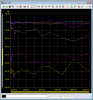
While on the subject of S/PDIF, let’s run another fun test. Remember what I said at the start of this article: our sources are the master. They generate the clock timing that the receiver must follow. While we want the receiver to follow the source, we only want it to do so with respect to generally playing the right number of samples per second. Ideally, it would not chase the errors induced by the cable or noise/distortion variations in the source. DACs implement a clock extraction/generation circuit called PLL. The PLL can be designed to filter out these variations. There are industry recommendations for both professional and consumer digital audio connections to do exactly that. It calls for a lot of filtering at higher frequencies (where it is easier) and reasonable amount at lower frequencies.
For grins, I decided to test the performance of a handful of devices to see how well they do in this respect. For this testing I used the Audio Precision Analyzer as the source since it is able to inject jitter at a specific frequency. By sweeping the jitter frequency from high to low and measuring the output of the DAC, we can determine if the above guideline is implemented. Here is what we get:
Starting from the bottom and going up, we have the Mark Levinson No 360S DAC in yellow, the Mark Levinson No 502 Processor in pink, then the Lexicon 12B in brown, and then a bunch of AVRs clustered around the zero line. Remember this is a log scale. So 60 dB means 1,000,000 times more attenuation than 0 dB. That is what the Mark Levinson DAC achieved. The Mark Levinson and Lexicon processors also did an excellent to good job of reducing jitter respectively.
Unfortunately the AVRs just sat there and took it all in. Not good. Not good at all. Translating, even when it comes to S/PDIF we are finding sloppy engineering in mass market devices. You better use very clean sources like I did with the Berkeley USB adapter. That device has an ultra-clean clock source and high isolation from the PC and therefore has much less reliance on the target device to clean up its signal. If you have an AVR, using a high quality asynchronous USB to S/PDIF adapter may be one of the best “tweaks” you can use to improve its performance (for music applications).
A Note on Audibility
I have shown you a lot of graphs but it would be unfair to leave them be as is. A lot of the distortions we see with HDMI are centered close to our main excitation frequency. When the distortions are close to a loud signal, and our source certainly is one in this case, they can’t be heard. So mostly like these are not audible distortions. As we get farther from the main tones, the spikes can reach higher than level of audibility and the chance of this occurring with HDMI is higher than with S/PDIF.
Summary and Final Thoughts
Digital audio is a complex area of audio. Characterizing its performance requires a good understanding of how it works, going beyond common misconceptions of it being “bit perfect.” The measurements show that HDMI is a setback from a performance point of view. While “heroic” efforts such as the Mark Levinson 502 manage to get superlative performance out of HDMI, it clearly presents a tough situation for lesser designs. More concerning is that the mere connection of a device to an HDMI source can cause it to degrade its performance over other inputs. Other anomalies include performance that is dynamic in ways that is not common in consumer electronic products.
Stand-alone dedicated devices such as the Mark Levinson DAC, the Peachtree decco65, and the Berkeley Audio Design Alpha USB interface show that when engineers focus on producing better quality they indeed get there, albeit at premium prices.
Sadly we did not find evidence of time making things better. Older products such as the aforementioned Mark Levinsons and Lexicon ran circles from a measurement point of view around the newer devices. Clearly this is another example of digital audio not following other digital technologies such as computers.
My advice is that if you are using your system for critical music listening, use S/PDIF instead of HDMI. If you are using a PC or Mac as the source, invest in a high-quality USB to S/PDIF converter.
As you may have noticed, I have not disclosed the identity of the systems that did not perform well here. My hope is that these companies take notice and improve their designs. It used to cost a lot for such instrumentation and hence the testing that I performed. In today’s dollars, my Audio Precision would set you back $30,000+. But innovations like the Prism Sound dScope have changed this landscape considerably. The version I used costs $9,895 which should be next to nothing for companies developing consumer electronics for mass markets. Some careful attention to circuit design and a few more dollars in parts should get us better performance. Let’s hope the next time I test these products, we see much better results.
Note 1: The references to absolute noise floor in this article (e.g. 120 dbFS) are not strictly correct in that the noise floor is partly determined by the characteristics of the measurement (i.e. FFT process gain). So it is best to use these measurements to compare products to each other as they all use identical parameters used for each.
I would like to sincerely thank the team including Simon Woollard,Ian Heaton,Graham Boswell, and Doug Ordon at Prism Sound for the kind loan of the dScope III, and their helpful advice, without which this article would not have been possible. Additional thanks for their kind permission to use some of the graphics from their presentation.
References
"Performance Challenges in Audio Converter Design," Ian Dennis, Prism Sound Systems, AES 24th UK CONFERENCE 2011
“The Diagnostic and Solution of Jitter-related Problems in Digital Systems,” Julian Dunn and Ian Dennis, Prism Sound Systems, AES 96th Convention, 1994
“Considerations for Interfacing Digital Audio Equipment to the Standards AES-3, AES-5, AES-11,” Julian Dunn, Prism Sound, 10th International Conference: Images of Audio (September 1991)
“The Numerically-Identical CD Mystery-A Study in Perception Versus Measurement,” Lan Dennis, Julian Dunn, and Doug Carson, AES Conference: UK 12th Conference: The Measure of Audio (MOA) (April 1997)
“Audio Engineering and Psychoacoustics: Matching Signals to the Final Receiver, the Human Auditory System,” Eberhard Zwicker and U. Tilmann Zwicker, JAES Volume 39 Issue 3 pp. 115-126; March 1991
Amir Majidimehr is the founder of Madrona Digital (www.madronadigital.com) which specializes in custom home electronics. He started Madrona after he left Microsoft where he was the Vice President in charge of the division developing audio/video technologies. With more than 30 years in the technology industry, he brings a fresh perspective to the world of home electronics.
Attachments
Last edited:
") So thanks for posting it.
So thanks for posting it.