• WANTED: Happy members who like to discuss audio and other topics related to our interest. Desire to learn and share knowledge of science required. There are many reviews of audio hardware and expert members to help answer your questions. Click here to have your audio equipment measured for free!

Audio Technica AT-OC9XML

Helicopter

Major Contributor
Forum Donor
Joined
Aug 13, 2020
Messages
2,693
Likes
3,944
Location
Michigan
The MM vs MI vs MC thread is getting a bit long, and covers several subtopics on measurements, so I am making this thread to focus on the cartridge I got when I took interest over there.

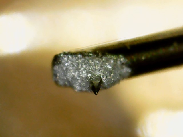
First, I figured a microscope inspection would be a good predecessor to ripping sweeps for measurement. Here's how my AT-OC9XML looks right now:

WIN_20210402_09_47_04_Pro.jpg


Obviously, my theory that the silver stuff around the stylus tip was protective packing grease or something like that was incorrect. It hasn't changed much with a couple hundred hours of break in and corresponding cleaning with melamine foam and a carbon fiber brush... anyway, looks clean enough, so time to rip some tracks and see if I can process them into useful data.
 

DSJR

Major Contributor
Joined
Jan 27, 2020
Messages
3,314
Likes
4,427
Location
Suffolk Coastal, UK
I was sad the previous At F2 and F7 had been discontinued, as I fondly remember the old and rather 'wild' F3 and F5 of old. Makes sense to use one basic boddy and generator for different stylus types which they've done so well with their VM95 and VM5**/7** ranges. Apparently, the sub £300 OC9XEN is a goodie and I bet the bonded elliptical ain't too shabby either.

AT aren't always the neatest in applying adhesive, but the diamonds usually seem good however. I have here an OC30 (more 'balls' than the old OC9's had) where the butt-mounted diamond has been knocked off, leaving a quantity of adhesive not so different to yours..

As for run-in, the old models asked for 1.5g tracking. I found that 1.7g or so for the first few album,s and then reducing to 1.5g as recommended then helped no end. Modern ones are 2g, so no idea now...
 
OP
Helicopter

Helicopter

Major Contributor
Forum Donor
Joined
Aug 13, 2020
Messages
2,693
Likes
3,944
Location
Michigan
I went straight from a Technics SL-1200 MK5 to a Focusrite Scarlett 2i2, with a Neutrik NC-MX RCA-XLR adapter and no phono preamp. I recorded the left channel only with CBS Test Record STR-100 track A1A left channel sweep, deleted everything before and after the sweep, and exported it as a signed 16-bit PCM .wav, which required down sampling and converting to stereo. That raw .wav file is published here.
 

JP

Major Contributor
Joined
Jul 4, 2018
Messages
2,274
Likes
2,449
Location
Brookfield, CT
I went straight from a Technics SL-1200 MK5 to a Focusrite Scarlett 2i2, with a Neutrik NC-MX RCA-XLR adapter and no phono preamp. I recorded the left channel only with CBS Test Record STR-100 track A1A left channel sweep, deleted everything before and after the sweep, and exported it as a signed 16-bit PCM .wav, which required down sampling and converting to stereo. That raw .wav file is published here.

Helicopter_AT-OC9XML.png
 

Tom C

Major Contributor
Joined
Jun 16, 2019
Messages
1,501
Likes
1,370
Location
Wisconsin, USA
Is a distortion analysis possible?
I’m surprised by the spectrum analysis. I would have expected a rising high frequency response, especially without RIAA correction.
I was too slow. JPJ has already posted...
 

Balle Clorin

Major Contributor
Joined
Dec 26, 2017
Messages
1,285
Likes
1,184
I took your file and compensated for pink noise slope and NO RIAA above 1 khz, constant velocity. Suspicious that right and left channels are identical when I tried to import to REW
1617379455638.png
 

JP

Major Contributor
Joined
Jul 4, 2018
Messages
2,274
Likes
2,449
Location
Brookfield, CT
I’m surprised by the spectrum analysis. I would have expected a rising high frequency response, especially without RIAA correction.

STR-100 sweep tracks are constant velocity from 500Hz. The 2i2 isn't going to load the cartridge right, so there will be some difference from that.
 

Balle Clorin

Major Contributor
Joined
Dec 26, 2017
Messages
1,285
Likes
1,184
Compared with my ATOC9 mkII/ML and Elipson test record sweep with 500R-0 eq, 200 ohms, and converted to linear RTA plot. Testrecords are likely to differ, see bottom plot
1617380467345.png


1617381002760.png
 
Last edited:
OP
Helicopter

Helicopter

Major Contributor
Forum Donor
Joined
Aug 13, 2020
Messages
2,693
Likes
3,944
Location
Michigan
Thanks! Interesting. Agree loading is off. Here is another raw recording with de-emphasis straight from my 100 ohm 180pF NAD PP2.

Would I need to buy Matlab to get Anaconda/Python to make the charts or am I just formatting the file names and locations incorrectly?

Code:
"""
PLEASE READ
To use this script you need to edit HOME to the directory where the .wav file is.
The .wav file can be any monotonic frequency sweep either up or down in frequency but
it must be trimmed at both ends to remove any leading silence. Frequencies below 1kHz are
ignored since virually all cartridges are well behaved below 1kHz.
Python does not read 24bit packed .wav's 16 bit is more than enough here.

The info_line should be alpha-numeric with entries separated by " / " only.  The script
will save a .png file that is named from the info line, replacing " / " with "_".  As
example "this / is / a / test" will create a file named "this_is_a_test.png"
"""

from scipy import signal
from scipy.io.wavfile import read
import matplotlib.pyplot as plt
import numpy as np
import datetime
import os

#edit here to add a HOME directory, etc.
HOME = 'Users\16073\Documents\Audacity'

_FILE = 'oc9xml.wav'
info_line =  'oc9xml'

#end edit

try:
    input = raw_input
except NameError:
    pass

#_FILE = input('Enter a .wav file (no quotes): ') #file needs to be >= sec_per_rev*2


#Needed to steal Matlab's flat top window

def ft_window(n):
    w = []
    a0 = 0.21557895
    a1 = 0.41663158
    a2 = 0.277263158
    a3 = 0.083578947
    a4 = 0.006947368
    pi = np.pi

    for x in range(0,n):
        w.append(a0 - a1*np.cos(2*pi*x/(n-1)) + a2*np.cos(4*pi*x/(n-1)) - a3*np.cos(6*pi*x/(n-1)) + a4*np.cos(8*pi*x/(n-1)))
    return w

try:
    input = raw_input
except NameError:
    pass

#_FILE = input('Enter a .wav file to process ')
#File needs trimming with no leading or trailing silence (undefined f)

y = read(HOME + _FILE)
Fs = float(y[0])
input_sig = y[1]

frequency = []
amplitude = []

frequency2h = []
amplitude2h = []

frequency3h = []
amplitude3h = []

freqout = []
ampout = []

freqout2h = []
ampout2h = []

freqout3h = []
ampout3h = []

F = int(Fs/100)
win = ft_window(F)

#For Fs sampling use small Fs/100 FFT's so frequency is f/100
#All common sampling rates are divisible by 100
#First try, no overlap and flat top window

#Find the minimum and maximum frequencies and flip the data if the sweep
#is going down in frequency.

y = abs(np.fft.rfft(input_sig[0:F]*win))
minf = np.argmax(y)

y = abs(np.fft.rfft(input_sig[len(input_sig)-F:len(input_sig)]*win))
maxf = np.argmax(y)

if maxf < minf:
    maxf,minf = minf,maxf
    input_sig = np.flipud(input_sig)


for x in range(0,len(input_sig)-F,F):
    y = abs(np.fft.rfft(input_sig[x:x+F]*win))
    f = np.argmax(y) #use largest bin
    if f >=10:
        frequency.append(f*100)
        amplitude.append(y[f])
    if 2*f<F/2-2 and f >= 10:
        f2 = np.argmax(y[(2*f)-2:(2*f)+2])
        frequency2h.append(f*100)
        amplitude2h.append(y[2*f-2+f2])
    if 3*f<F/2-2 and f >= 10:
        f3 = np.argmax(y[(3*f)-2:(3*f)+2])
        frequency3h.append(f*100)
        amplitude3h.append(y[3*f-2+f3])

amp = 0
count = 0
x = minf*100

for x in range(minf*100,(maxf+1)*100,100):
    for y in range(0,len(frequency)):
        if frequency[y] == x:
            amp = amp + amplitude[y]
            count = count + 1
    if count != 0:
        freqout.append(x)
        ampout.append(20*np.log10(amp/count))
    amp = 0
    count = 0

amp = 0
count = 0
x = minf*100

for x in range(minf*100,(maxf+1)*100,100):
    for y in range(0,len(frequency2h)):
        if frequency2h[y] == x:
            amp = amp + amplitude2h[y]
            count = count + 1
    if count != 0:
        freqout2h.append(x)
        ampout2h.append(20*np.log10(amp/count))
    amp = 0
    count = 0
   

amp = 0
count = 0
x = minf*100

for x in range(minf*100,(maxf+1)*100,100):
    for y in range(0,len(frequency3h)):
        if frequency3h[y] == x:
            amp = amp + amplitude3h[y]
            count = count + 1
    if count != 0:
        freqout3h.append(x)
        ampout3h.append(20*np.log10(amp/count))
    amp = 0
    count = 0


b, a = signal.iirfilter(3,.5, btype='lowpass') #filter some noise
ampout = signal.filtfilt(b,a,ampout)
ampout2h = signal.filtfilt(b,a,ampout2h)
ampout3h = signal.filtfilt(b,a,ampout3h)

norm = ampout[0]
ampout = ampout-norm #amplitude is in dB so normalize by subtraction at [0]
ampout2h = ampout2h-norm
ampout3h = ampout3h-norm

f, plt.figure(figsize=(14,6))
plt.semilogx(freqout,ampout,color = 'b')
plt.semilogx(freqout2h,ampout2h,color = 'g')
plt.semilogx(freqout3h,ampout3h,color = 'r')
plt.grid(True, which="both", axis="x", ls="-", color="black")
plt.grid(True, which="major", axis="both", ls="-", color="black")
plt.grid(True, which="minor", axis="both", ls="-", color="gainsboro")
#plt.grid(True, which="both", axis="x", ls="-", color="black")
#plt.xaxis.grid(True, which="minor", ls="-", color="gainsboro")
plt.minorticks_on()
plt.title("Instantaneous Frequency vs. Amplitude and Distortion: "+ _FILE + "\n", fontsize=16)
plt.xlabel("Frequency (Hz)")
plt.ylabel("Amplitude (dB)")

plt.figtext(.17,.7,'- 2nd harmonic -',color = 'g')
plt.figtext(.17,.67,'- 3rd harmonic -',color = 'r')

plt.tick_params(which='both',
                top='off',
                left='off',
                right='off',
                bottom='off')

mod_date = datetime.datetime.fromtimestamp(os.path.getmtime(_FILE))

plt.figtext(.17, .13, info_line + "\n" + \
            mod_date.strftime("%b %d, %Y %H:%M:%S"), fontsize=10)
         
plt.savefig(info_line.replace(' / ', '_') +'.png', bbox_inches='tight', pad_inches=.75, dpi=96)

#plt.show()
 

JP

Major Contributor
Joined
Jul 4, 2018
Messages
2,274
Likes
2,449
Location
Brookfield, CT
Don't need to buy anything. Just need Python and to install the libraries (matplotlib, scipy, and numpy). The latest version of the script *should* be OS independent, but I've not tried it on Windows.
 
OP
Helicopter

Helicopter

Major Contributor
Forum Donor
Joined
Aug 13, 2020
Messages
2,693
Likes
3,944
Location
Michigan
I took your file and compensated for pink noise slope and NO RIAA above 1 khz, constant velocity. Suspicious that right and left channels are identical when I tried to import to REW
View attachment 121621
I made a mono recording, left channel only, and then when I convert it to wav it gets down sampled and converted to stereo.
 

JP

Major Contributor
Joined
Jul 4, 2018
Messages
2,274
Likes
2,449
Location
Brookfield, CT
Thanks! Interesting. Agree loading is off. Here is another raw recording with de-emphasis straight from my 100 ohm 180pF NAD PP2.

Would I need to buy Matlab to get Anaconda/Python to make the charts or am I just formatting the file names and locations incorrectly?

Code:
"""
PLEASE READ
To use this script you need to edit HOME to the directory where the .wav file is.
The .wav file can be any monotonic frequency sweep either up or down in frequency but
it must be trimmed at both ends to remove any leading silence. Frequencies below 1kHz are
ignored since virually all cartridges are well behaved below 1kHz.
Python does not read 24bit packed .wav's 16 bit is more than enough here.

The info_line should be alpha-numeric with entries separated by " / " only.  The script
will save a .png file that is named from the info line, replacing " / " with "_".  As
example "this / is / a / test" will create a file named "this_is_a_test.png"
"""

from scipy import signal
from scipy.io.wavfile import read
import matplotlib.pyplot as plt
import numpy as np
import datetime
import os

#edit here to add a HOME directory, etc.
HOME = 'Users\16073\Documents\Audacity'

_FILE = 'oc9xml.wav'
info_line =  'oc9xml'

#end edit

try:
    input = raw_input
except NameError:
    pass

#_FILE = input('Enter a .wav file (no quotes): ') #file needs to be >= sec_per_rev*2


#Needed to steal Matlab's flat top window

def ft_window(n):
    w = []
    a0 = 0.21557895
    a1 = 0.41663158
    a2 = 0.277263158
    a3 = 0.083578947
    a4 = 0.006947368
    pi = np.pi

    for x in range(0,n):
        w.append(a0 - a1*np.cos(2*pi*x/(n-1)) + a2*np.cos(4*pi*x/(n-1)) - a3*np.cos(6*pi*x/(n-1)) + a4*np.cos(8*pi*x/(n-1)))
    return w

try:
    input = raw_input
except NameError:
    pass

#_FILE = input('Enter a .wav file to process ')
#File needs trimming with no leading or trailing silence (undefined f)

y = read(HOME + _FILE)
Fs = float(y[0])
input_sig = y[1]

frequency = []
amplitude = []

frequency2h = []
amplitude2h = []

frequency3h = []
amplitude3h = []

freqout = []
ampout = []

freqout2h = []
ampout2h = []

freqout3h = []
ampout3h = []

F = int(Fs/100)
win = ft_window(F)

#For Fs sampling use small Fs/100 FFT's so frequency is f/100
#All common sampling rates are divisible by 100
#First try, no overlap and flat top window

#Find the minimum and maximum frequencies and flip the data if the sweep
#is going down in frequency.

y = abs(np.fft.rfft(input_sig[0:F]*win))
minf = np.argmax(y)

y = abs(np.fft.rfft(input_sig[len(input_sig)-F:len(input_sig)]*win))
maxf = np.argmax(y)

if maxf < minf:
    maxf,minf = minf,maxf
    input_sig = np.flipud(input_sig)


for x in range(0,len(input_sig)-F,F):
    y = abs(np.fft.rfft(input_sig[x:x+F]*win))
    f = np.argmax(y) #use largest bin
    if f >=10:
        frequency.append(f*100)
        amplitude.append(y[f])
    if 2*f<F/2-2 and f >= 10:
        f2 = np.argmax(y[(2*f)-2:(2*f)+2])
        frequency2h.append(f*100)
        amplitude2h.append(y[2*f-2+f2])
    if 3*f<F/2-2 and f >= 10:
        f3 = np.argmax(y[(3*f)-2:(3*f)+2])
        frequency3h.append(f*100)
        amplitude3h.append(y[3*f-2+f3])

amp = 0
count = 0
x = minf*100

for x in range(minf*100,(maxf+1)*100,100):
    for y in range(0,len(frequency)):
        if frequency[y] == x:
            amp = amp + amplitude[y]
            count = count + 1
    if count != 0:
        freqout.append(x)
        ampout.append(20*np.log10(amp/count))
    amp = 0
    count = 0

amp = 0
count = 0
x = minf*100

for x in range(minf*100,(maxf+1)*100,100):
    for y in range(0,len(frequency2h)):
        if frequency2h[y] == x:
            amp = amp + amplitude2h[y]
            count = count + 1
    if count != 0:
        freqout2h.append(x)
        ampout2h.append(20*np.log10(amp/count))
    amp = 0
    count = 0
 

amp = 0
count = 0
x = minf*100

for x in range(minf*100,(maxf+1)*100,100):
    for y in range(0,len(frequency3h)):
        if frequency3h[y] == x:
            amp = amp + amplitude3h[y]
            count = count + 1
    if count != 0:
        freqout3h.append(x)
        ampout3h.append(20*np.log10(amp/count))
    amp = 0
    count = 0


b, a = signal.iirfilter(3,.5, btype='lowpass') #filter some noise
ampout = signal.filtfilt(b,a,ampout)
ampout2h = signal.filtfilt(b,a,ampout2h)
ampout3h = signal.filtfilt(b,a,ampout3h)

norm = ampout[0]
ampout = ampout-norm #amplitude is in dB so normalize by subtraction at [0]
ampout2h = ampout2h-norm
ampout3h = ampout3h-norm

f, plt.figure(figsize=(14,6))
plt.semilogx(freqout,ampout,color = 'b')
plt.semilogx(freqout2h,ampout2h,color = 'g')
plt.semilogx(freqout3h,ampout3h,color = 'r')
plt.grid(True, which="both", axis="x", ls="-", color="black")
plt.grid(True, which="major", axis="both", ls="-", color="black")
plt.grid(True, which="minor", axis="both", ls="-", color="gainsboro")
#plt.grid(True, which="both", axis="x", ls="-", color="black")
#plt.xaxis.grid(True, which="minor", ls="-", color="gainsboro")
plt.minorticks_on()
plt.title("Instantaneous Frequency vs. Amplitude and Distortion: "+ _FILE + "\n", fontsize=16)
plt.xlabel("Frequency (Hz)")
plt.ylabel("Amplitude (dB)")

plt.figtext(.17,.7,'- 2nd harmonic -',color = 'g')
plt.figtext(.17,.67,'- 3rd harmonic -',color = 'r')

plt.tick_params(which='both',
                top='off',
                left='off',
                right='off',
                bottom='off')

mod_date = datetime.datetime.fromtimestamp(os.path.getmtime(_FILE))

plt.figtext(.17, .13, info_line + "\n" + \
            mod_date.strftime("%b %d, %Y %H:%M:%S"), fontsize=10)
       
plt.savefig(info_line.replace(' / ', '_') +'.png', bbox_inches='tight', pad_inches=.75, dpi=96)

#plt.show()


That's an older version of the script. Home is in Mac/UNIX directory nomenclature. I also had to trim the first ~7 seconds off your file as the amplitude was too low there.
 

DSJR

Major Contributor
Joined
Jan 27, 2020
Messages
3,314
Likes
4,427
Location
Suffolk Coastal, UK
That response looks ok to me. A dB or two lift over 10khz seems a feature of modern far eastern cartridges except those intended for vintage audio people. I was told once that Japanese vinyl had a softer compound and maybe softer highs as well, which is why many japanese cartridges liked a lifted hf and in older models, a steeper diamond rake angle not really fixed with VTA adjustment.
 
OP
Helicopter

Helicopter

Major Contributor
Forum Donor
Joined
Aug 13, 2020
Messages
2,693
Likes
3,944
Location
Michigan
This code:

Code:
from scipy import signal
from scipy.io.wavfile import read
import matplotlib.pyplot as plt
import numpy as np

#edit here to add a HOME directory
#HOME = "/home/david/"  #Linux example
HOME = 'C:\Users\16073\Documents\Audacity\' #Windows example
#edit here for 45 rpm samples
Period = 1.8 # 33rpm
#Period = 4/3 # 45 rpm
#end edit

def instfreq(sig,Fs):
    z = signal.hilbert(sig)
    rawfreq = Fs/(2*np.pi)*np.diff(np.unwrap(np.angle(z)))
    rawfreq = np.append(rawfreq,rawfreq[len(rawfreq)-1])    #np.diff drops one end point
    b, a = signal.iirfilter(1,100./(Fs/2), btype='lowpass')
    a = np.convolve(a,a) #make an ordinary 100Hz 4 pole filter.
    a = np.convolve(a,a)
    b = np.convolve(b,b)
    b = np.convolve(b,b)
    instfreq = signal.lfilter(b,a,rawfreq)
    return (instfreq)

_FILE = input('oc9xml.wav') #file needs to be >= 4 sec.

y = read(HOME + _FILE)
Fs = float(y[0])
if np.size(y[1][0]) == 2:
    sig = y[1][:,0][0:int(Fs*4)] #Grab 4 sec of a stereo file from the first (left?) channel
else:
    sig = y[1][0:int(Fs*4)] #mono file

t = np.arange(Period,0,-1/Fs)  #Reverse time (theta axis)
theta = t*2*np.pi/Period   #Time becomes degrees (Periodsec = 2pi radians)
theta = np.roll(theta,int(Fs*.45))  #Rotate 90 deg to put 0 on top (Period*Fs/4)

freq1 = instfreq(sig,Fs)
glitch = 2000   #remove leading glitch from output (probably should depend on Fs)
if1 = freq1[glitch:glitch+int(Fs*Period)] 
if2 = freq1[glitch+int(Fs*Period):glitch+int(2*Fs*Period)]
          
maxf = int(max(max(if1),max(if2))+.5)

r1 = 20.-(maxf-if1)/3.  #20 radial ticks at 3Hz is fixed, adaptive scaling
r2 = 20.-(maxf-if2)/3.  #is an exercise for later


ax = plt.subplot(111, projection='polar')
ax.plot(theta,r1)
ax.plot(theta,r2)
ax.set_rmax(20)
                        #Set up the ticks y is radial x is theta, it turns out x and y
                        #methods work in polar projection but sometimes do funny things

for tick in ax.yaxis.get_major_ticks():
                tick.label.set_fontsize(8)
plt.yticks(np.arange(1,21,1))
ax.set_rlabel_position(90)

myticks = []   
for x in range(0,20,1):
    myticks.append(str(maxf-57+x*3))
ax.set_yticklabels(myticks)

ax.set_xticklabels(['90'+u'\N{DEGREE SIGN}','45'+u'\N{DEGREE SIGN}','0'+u'\N{DEGREE SIGN}',\
                    '315'+u'\N{DEGREE SIGN}','270'+u'\N{DEGREE SIGN}','225'+u'\N{DEGREE SIGN}',\
                    '180'+u'\N{DEGREE SIGN}','135'+u'\N{DEGREE SIGN}'])
ax.grid(True)

ax.set_title("Instantaneous Frequency  "+ _FILE, va='bottom')
plt.show()

spits out this figure now:

1617383625755.png


I guess that's an improvement. :D
 

JP

Major Contributor
Joined
Jul 4, 2018
Messages
2,274
Likes
2,449
Location
Brookfield, CT
That's the polar plot code, not the FR code.
 

JP

Major Contributor
Joined
Jul 4, 2018
Messages
2,274
Likes
2,449
Location
Brookfield, CT

JP

Major Contributor
Joined
Jul 4, 2018
Messages
2,274
Likes
2,449
Location
Brookfield, CT
This is an inverse RIAA filter you can use in Audacity to remove EQ when recording with your phono stage. Select the audio, go to Tools, Nyquist Prompt, and enter this. Also check the v3 syntax box. It's for 44.1 sample rate only.

Code:
(biquad-m s 7.424809e+000 -1.285961e+001 5.448569e+000 1.000000e+000 -9.311757e-001 0.000000e+000)

Screen Shot 2021-04-02 at 3.20.51 PM.png
 
OP
Helicopter

Helicopter

Major Contributor
Forum Donor
Joined
Aug 13, 2020
Messages
2,693
Likes
3,944
Location
Michigan
This is an inverse RIAA filter you can use in Audacity to remove EQ when recording with your phono stage. Select the audio, go to Tools, Nyquist Prompt, and enter this. Also check the v3 syntax box. It's for 44.1 sample rate only.

Code:
(biquad-m s 7.424809e+000 -1.285961e+001 5.448569e+000 1.000000e+000 -9.311757e-001 0.000000e+000)

View attachment 121651
This works fine for me, but I can't get the script to work in Anaconda. I ran

conda install matplotlib

conda install scipy

conda install numpy

and all they all went through without erroring out. However, that polar plot code is the only thing I have been able to get to generate anything.
 
Top Bottom