Bass and subwoofers

[audiofooled]

I just ran about 30 tracks through matlab. Clunky, slow. I filtered the L and R to 60Hz, with a filter cutting off by 80dB at 120Hz. (long FIR constant delay filter) and then rudely calculated the normalized cross-correlation between the two channels ( this means I ignored level differences, but captured all changes due to phase, frequency, etc).

This is a number that can vary between -1 and 1. -1 means that the two signals are precisely out of phase and identical (except for level). 1 means they are identical. 0 means they are uncorrelated.

Lowest number I saw was .2 on an acoustic recording with a multimike panpotted arrangement with widely spaced mikes. Unquestionably this did not do any "mix to mono". A bunch of pop recordings came in very precisely at .95 +- .02. A LOT of them. That's actually kind of weird, because they are "almost mono bass". I'd say 50% were above .9 and about 10% under .5. I didn't find any track overall that was under 0. Out of about 30 tracks, only ONE hit '1'. No, it wasn't a mono recording.

Now, this is a very, very rough, broad approximation, it's 2AM, I was bored, and I did the fastest (by code writing) calculation I could imagine. I will go back and do more like I did long ago, calculating both level and phase mismatch, zero out quiet parts, and get a histogram of the actual "sameness" <or lack thereof>. But not tonight. Since this very broad measure would tend to hide differences in level, I'll have to say that there is much less mono bass in modern recordings.

Is there a chance to not exclude tracks where most of the bass is mono (usually in the band of 40-80Hz), but sense of space/decorrelation is latent in low level signals bellow 30hz, sometimes even 20?

 

[NTK]

If I have not misunderstood Dr Griesinger, stereo bass is necessary but not sufficient for envelopment, and there isn't a simple measurement.
(Source: http://www.davidgriesinger.com/laaes2.pdf, slides 27 & 28)

He names his brute force method "DFT" (diffuse field transfer function).

Here are the more detailed descriptions of the steps in his proposed method:
(From: http://www.davidgriesinger.com/overvw1.pdf pages 7-8)

... Using this algorithm and a narrow band noise signal as a test probe we developed our measure for envelopment in small rooms. We call it the DFT, or diffuse field transfer function.​

​

The process of finding the diffuse field transfer function can be summarized:​

1. Calculate (or measure) separate binaural impulse responses for each loudspeaker position to a particular listener position. A high sample rate must be chosen to maintain timing accuracy. In our experiments 176400Hz is an adequate sample rate.
2. Low-pass filter each impulse response and resample at 11025Hz, and then do it again, ending with a sample rate of 2756Hz. This sample rate is adequate for the frequencies of interest, and low enough that the convolutions do not take too much time.
3. Create a test signals from independent filtered noise signals. Various frequencies and bandwidths can be tried, depending on the correlation time of the musical signal of interest.
4. Convolve each binaural impulse response with a different band filtered noise signal, and sum the resulting convolutions to derive the pressure at each ear.
5. Extract the ITD from the two ear signals by comparing the positive zero-crossing time of each cycle.
6. Average the ITDs thus extracted to find the running average ITD. The averaging process weights each ITD by the instantaneous pressure amplitude. In other words, ITDs where the amplitudes at the two ears is high count more strongly in the average than ITDs where the amplitude is low.
7. Sum the running average ITD and divide by the length to find the average ITD and the apparent azimuth of the sound source.
8. Subtract the average value from the running average ITD to extract the interaural fluctuations.
9. Filter the result with a 3Hz to 17Hz bandpass filter to find the fluctuations that produce envelopment.
10. Measure the strength of these fluctuations by finding the average absolute value of the fluctuations. The number which results is the Diffuse Field Transfer function, or DFT.
11. Measure the DFT as a function of the receiver position in the room under test.

 

[bmc0]

I filtered the L and R to 60Hz, with a filter cutting off by 80dB at 120Hz. (long FIR constant delay filter) and then rudely calculated the normalized cross-correlation between the two channels
[...]
I will go back and do more like I did long ago, calculating both level and phase mismatch, zero out quiet parts, and get a histogram of the actual "sameness" <or lack thereof>

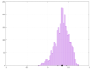
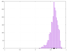
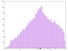
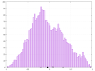
I was inspired by your post to write a small C program to compute the normalized cross-correlation over a specified window. The chunks overlap (hop is set to 1/16th the chunk length) and are windowed using a half sine function. The program outputs a gnuplot script which produces a weighted (RMS of sample values) histogram along with some simple statistical info. Is this perhaps a reasonable/useful way of looking at the "stereo-ness"?

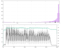
EDIT: Turns out I made a serious error, so it's probably best to disregard the plots below... Stay tuned for an update. I can write code, but I know virtually nothing about statistics
Edit 2: See post #207.

---

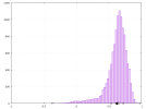
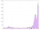
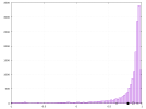
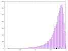
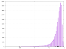
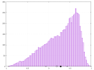
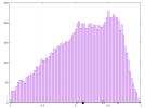
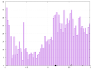
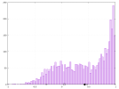
Below are some example plots using an 8th-order butterworth lowpass at 80Hz and a window of 500ms. The filled circle along the x-axis is the weighted mean.
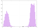
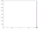
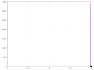
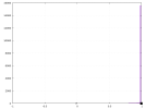
Mono pink noise:

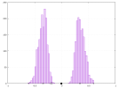
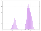
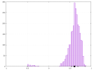
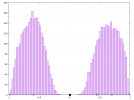
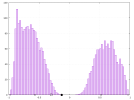
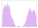
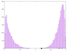
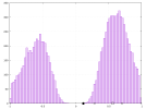
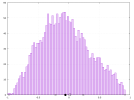
Correlation of 1, as expected. Stereo pink noise (uncorrelated), then with the side channel attenuated by 3dB and 6dB (increasing positive correlation):

Shows a bimodal distribution with the weighted mean being close to 0 (-0.0037) for the uncorrelated case.
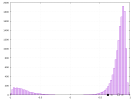
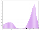
Here's the RCA Reiner/CSO recording of Scheherazade mentioned in post #199 (entire work, not just the first movement):

Debussy's La Mer from the same CD:

Here are the two tracks I posted XY display videos of in post #147:

An interesting one—"Hunter" by Björk:

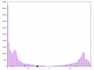
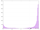
Most of the bass is out of phase! Many of the other tracks on that album have basically mono bass. Here's Alarm Call (weighted mean = 0.996):

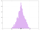
Here's "Truth Lies Low" by Andrew Bird (weighted mean = 0.557):

Many of the other tracks from that album have significantly higher correlation.
A few more orchestral recordings (Decca and Telarc):

 

[LIΟN]

I was inspired by your post to write a small C program to compute the normalized cross-correlation over a specified window. The chunks overlap (hop is set to 1/16th the chunk length) and are windowed using a half sine function. The program outputs a gnuplot script which produces a weighted (RMS of sample values) histogram along with some simple statistical info. Is this perhaps a reasonable/useful way of looking at the "stereo-ness"?

EDIT: Turns out I made a serious error, so it's probably best to disregard the plots below... Stay tuned for an update. I can write code, but I know virtually nothing about statistics

Below are some example plots using an 8th-order butterworth lowpass at 80Hz and a window of 500ms. The filled circle along the x-axis is the weighted mean.
Mono pink noise:
View attachment 435337
Correlation of 1, as expected. Stereo pink noise (uncorrelated), then with the side channel attenuated by 3dB and 6dB (increasing positive correlation):
View attachment 435339View attachment 435340View attachment 435341
Shows a bimodal distribution with the weighted mean being close to 0 (-0.0037) for the uncorrelated case.
Here's the RCA Reiner/CSO recording of Scheherazade mentioned in post #199 (entire work, not just the first movement):
View attachment 435342
Debussy's La Mer from the same CD:
View attachment 435344
Here are the two tracks I posted XY display videos of in post #147:
View attachment 435345View attachment 435346
An interesting one—"Hunter" by Björk:
View attachment 435347
Most of the bass is out of phase! Many of the other tracks on that album have basically mono bass. Here's Alarm Call (weighted mean = 0.996):
View attachment 435348
Here's "Truth Lies Low" by Andrew Bird (weighted mean = 0.557):
View attachment 435350
Many of the other tracks from that album have significantly higher correlation.
A few more orchestral recordings (Decca and Telarc):
View attachment 435351View attachment 435352View attachment 435353View attachment 435354

Really nice. Could you share the program you created?

 

[bmc0]

Could you share the program you created?

Sure, after I figure out the correct way of doing things .
In the post above, I had the program search for the maximum absolute value of the cross-correlation, but 1) I didn't realize that the output (computed via FFT) is circularly shifted, so it turns out that it was only looking at positive lags (negative time shift), and 2) on second thought, searching for maximum correlation over such a large time window is probably not what should be done.
The first explains the preponderance of chunks with high negative correlation with the Björk track—upon further inspection, the bass isn't mostly out of phase.

 

[j_j]

Doing this on 50-100 millisecond windows makes more sense than the one size fits all calculation I did.

Maybe I'll write something to iterate over appropriate block lengths with a Hann window and see what crawls out.

 

[bmc0]

Okay, take 2 of post #203... I think it's working correctly. It only looks at the zero lag data point now. Not sure if it makes sense to search within a limited window or not.

New plots in the same order as before (same 500ms window and 8th-order Butterworth lowpass at 80Hz):
Pink noise—mono, stereo, side at -3dB, and side at -6dB:

No more bimodal distribution.
RCA Reiner/CSO recording of Scheherazade mentioned in post #199 (entire work, not just the first movement) and Debussy's La Mer from the same CD:

The two tracks I posted XY display videos of in post #147:

"Hunter" and "Alarm Call" by Björk:

"Truth Lies Low" by Andrew Bird:

A few more orchestral recordings (Decca and Telarc):


Edit: Bonus tracks—"The Moment I Said It" and "2-1", both by Imogen Heap:

 

[bmc0]

Doing this on 50-100 millisecond windows makes more sense than the one size fits all calculation I did.

Is there a reason to use a window this short? I'm asking since I really have no idea what might be optimal . With the few tracks I tested, a 100ms window seems to result in a wider peak in the histograms than 500ms but generally gives similar mean values.

 

[j_j]

Is there a reason to use a window this short? I'm asking since I really have no idea what might be optimal . With the few tracks I tested, a 100ms window seems to result in a wider peak in the histograms than 500ms but generally gives similar mean values.

Well, the two time constants in the auditory system that might make sense are the 100ms and about 2 seconds. I think that the 2 seconds will miss the point of envelopment, which has to change inside that window.

I just did some stuff on crosscorrelation and level. Trying to figure out how to present them, it's not amenable to one graph, I fear.

 

[LIΟN]

100ms and about 2 seconds.

Whenever you have a moment, like enjoying a cup of coffee, could you share a few small keywords regarding 100ms / 2s?
I truly appreciate all your contributions.

 

[gnarly]

Interesting webinar on smoothing out spatial response of multiple subs using phase decorrelation.
Geared towards live sound, but acoustics are acoustics. And I think it applies to muti-sub, and virtual-sub room reflections oh so well.

Vid changes from intro-type content to discuss the DSP phase decorrelation applied, at about 28min.

A take away/confirmation for me, was how spatial evenness was achieved through DSP phase and time decorrelation, but at the expense of impact.
This has been my experience every time I play with multiple subs.

Their solution? Monitor the music's impulse response... When sharp transients occur, turn off the DSP response smoothing algorithm for the duration of the transient.

 

[bmc0]

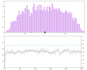
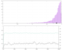
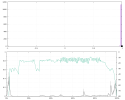
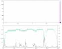
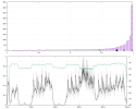
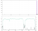
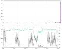
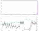
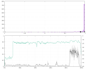
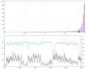
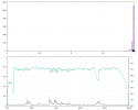
I've been playing around with calculating a crude "LF envelopment potential" metric vs time. Basically, I apply Griesinger's idea of ITD fluctuations to the short-time cross-correlation values along with some additional filtering to suppress some things I wouldn't expect to create envelopment. I'm making no strong claims about accuracy or robustness, but it seems to more-or-less correlate with what I hear in many cases.

A few examples using a 60ms window (Hann):

Stereo pink noise with correlation ~0 and ~0.83:

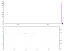
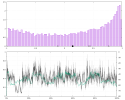
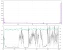
The upper plot is a weighted cross-correlation histogram. The bottom plot shows the RMS level (dB) of the observed band (20-80Hz) in green and my "LF envelopment potential" metric in gray (less smoothing) and black (more smoothing).
Mono pink noise:

No predicted envelopment (as it should be).
RCA Reiner/CSO recording of Scheherazade (first movement):

Somewhat difficult to interpret this one, I think.
Thomas Lund mentioned a particular Billie Eilish track a while back—

or listen to Billie Eilish’s I Didn’t Change My Number, where, in a bone-dry track, verses have correlated bass, developing into AE explosions in the choruses.

Let's have a look at that:

Seems to hint pretty well at what he's talking about. Another track from the same album with very little predicted envelopment, "my future":

"Hunter" and "Alarm Call" by Björk:

"Make Them Gold", "Get Away", and "High Enough to Carry You Over" by CHVRCHΞS:

"Exit Music (for a Film)" by Radiohead:

Predicted LF envelopment goes away during the climax.
"Roma Fade", "Truth Lies Low", and "Are You Serious" by Andrew Bird:


OK, I think that's enough for now.

 

[j_j]

The thing that I haven't fooled with yet is the level issue, which is also involved, I suspect the variation in arrival coupled with the energy is going to turn out to be the metric, but I've been busy doing retirement.

 

[bmc0]

The thing that I haven't fooled with yet is the level issue, which is also involved

My algorithm incorporates a very simple forward temporal masking model. It also suppresses spikes in the reported metric during rapid increases in level and when the channel levels are unbalanced. These take care of at least some of the unwanted noise, but I expect that coming up with a robust algorithm will be difficult (especially for me as I don't really know what I'm doing ).

Do you think that separating the input into multiple bands would be useful?

 

[j_j]

My algorithm incorporates a very simple forward temporal masking model. It also suppresses spikes in the reported metric during rapid increases in level and when the channel levels are unbalanced. These take care of at least some of the unwanted noise, but I expect that coming up with a robust algorithm will be difficult (especially for me as I don't really know what I'm doing ).

Do you think that separating the input into multiple bands would be useful?

Well, below 50Hz you're working at the very end of the basilar membrane, so grouping everything BELOW (thanks, bmc0) that might be reasonable. Above that, maybe 30Hz bands would suffice. The length of the required cochlear filters will rather point out the slowness of the mechanism, and you can hypothesize a 30dB below current level as a masking level, I'd think. Now leading edges should turn out to be the biggest contributor to actual perception, but I don't have any data handy on how much (and I suspect nobody does).

You may not think you're know what you're doing, but you're doing actual research, so don't put yourself down like that. If you can get something between 20 and 80Hz that corresponds to what you hear, frankly, you might consider publishing it.

 

[bmc0]

Thanks for the info and encouragement, @j_j; much appreciated. When I say "seems to correlate," that's just based on sighted listening of a few tracks so take that statement with a (large) grain of salt.

below 50Hz you're working at the very end of the basilar membrane, so grouping everything above that might be reasonable.

This should read "everything below [50Hz]", correct?

 

[j_j]

Thanks for the info and encouragement, @j_j; much appreciated. When I say "seems to correlate," that's just based on sighted listening of a few tracks so take that statement with a (large) grain of salt.


This should read "everything below [50Hz]", correct?

You are correct, and, of course, you will have to devise some way to run a blind test and compare "width" vs. your measure. Trust me, I know that's a pain in the butt.

 

[audiofooled]

Thomas Lund mentioned a particular Billie Eilish track a while back—

Let's have a look at that:
View attachment 436427
Seems to hint pretty well at what he's talking about.

Let's take a look of the portion of this track that actually contains high potential for envelopment (L-green, R-blue):

Zoom in a bit and take a look at L (green), R (blue) and mono (red):

It will strongly depend on how they do decorrelation on the production side, so that only "some information" is lost during mono summation, up to "almost everything is lost"- they don't want that. One thing for sure, potential for envelopment is lost entirely if we actually mono the signal.

For this reason of translation to various systems, most of the bass is mono most of the time, especially in the signals with highest crest factor, but not all of it - all the time.
IME, there are many tracks where stereo bass is latent in very low frequencies (also lower in level-so that small systems are completely oblivious to that, basically, it goes under the radar). Look for it lower than 40Hz.

 

[Thomas Lund]

- what are you thoughts on a speaker’s step function or impulse response? And phase in general?

Concerning inducement of AE, absolute LF time and phase isn’t important. It is inter-aural time that matters.

Whether or not loudspeakers should replicate reliably what microphones picked up, or what was built with level panning, I guess depends on application.

In monitoring, you want it to be so. Playback includes inter-aural evaluation; plus at least one requirement for absolute time: Group delay must be constant across cross-over points, at frequencies where listener movement is a factor. As active sensors, human adults reach out constantly to seek meaning. In sound, this involves head and body movement, e.g. to distinguish between direct sound and reflections of the listening room. Therefore, direct sound must never ever be contaminated the same way reflections naturally are; by modulated sound colour and/or time, as result of listener movement.

In recreational listening, it can be argued music should primarily rather sound nice and comforting.

 

[bmc0]

leading edges should turn out to be the biggest contributor to actual perception

Dr. Griesinger mentions extracting ITD from the positive-going zero crossings. Is that what you mean here, or something else?