Chord quest, Vs Rme adi-2 dac fs + tap count.

[Gurra1980]

Well it looks a lot more advanced than this. But is it really?

 

[Gurra1980]

Indeed, nothing wrong with it, just limited to the 5. If you have in-room measurements in REW, you can see how far you can get with 5 PEQ’s using the EQ tool.

Well I actually thought it was almost endless in its capabilities. I may have to rethink this. Thanks.

 

[voodooless]

It’s a shame you can’t use those tens of thousands of taps of Chord.. it would make for a very good DSP engine for room correction.

 

[LTig]

Well it looks a lot more advanced than this. But is it really? View attachment 122148

Yes it is. What you show is a fixed 5 band GEQ.

 

[Gurra1980]

Yes it is. What you show is a fixed 5 band GEQ.

Yes that's what I thought, so what you can do I guess is choose one of the five and then shape the curve around it? Is this correct?

 

[Gurra1980]

It’s a shame you can’t use those tens of thousands of taps of Chord.. it would make for a very good DSP engine for room correction.

Haha that would be great!

 

[Jimbob54]

Yes it is. What you show is a fixed 5 band GEQ.

And its 5 plus the 2 shelf filters. But as others have said, depends what the OP room needs and how far they want to go.

As regards the chord dacs vs any other well measuring example from these pages I suggest the OP buys one from amazon, does their own (level matched and reasonably well controlled) tests and flogs the chord if they can't discern the difference or returns the amazon one if the chord is audibly superior.

 

[LTig]

Yes that's what I thought, so what you can do I guess is choose one of the five and then shape the curve around it? Is this correct?

Yep. See here if you want to know more about what a PEQ can do.

 

[Jimbob54]

Yes that's what I thought, so what you can do I guess is choose one of the five and then shape the curve around it? Is this correct?

I think you need to find articles on using parametric eq. Simply put, for each of the bands you tell the device what frequency to vary, by how much and what gradient the curve is around that freq (how steep or broad the "hill" is around the freq)

Edit, hill or valley of course.

 

[voodooless]

If you want more EQ options, check out the Motu interfaces that can run as standalone units. The ultra lite MK4 is quite powerful, and within budget.

Edit: also the Motu only has a limited number of EQ’s available it seems is otherwise much more powerful though.

 

[Phorize]

The FPGA’s extraordinary capability enables a number of key sonic benefits, including significantly improved timing and the best noise-shaper performance of any known DAC. DAVE’s technology delivers music with unmatched reality and musicality, with an unrivalled timing response.

They claim it has sonic benefits, unmatched musicality and realism.

What do you believe is concrete or specific about claiming ‘sonic benefits’, ‘unmatched musicality’ or ‘realism’? I posit that these claims are in absolutely meaningless. Do you disagree? If so, I’d be genuinely interested as to why.

 

[Gurra1980]

What do you believe is concrete or specific about claiming ‘sonic benefits’, ‘unmatched musicality’ or ‘realism’? I posit that these claims are in absolutely meaningless. Do you disagree? If so, I’d be genuinely interested as to why.

Haha sorry, but I'm not really interested in debating who says what and why. Let's get back on topic

 

[Gurra1980]

If you want more EQ options, check out the Motu interfaces that can run as standalone units. The ultra lite MK4 is quite powerful, and within budget.

Edit: also the Motu only has a limited number of EQ’s available it seems is otherwise much more powerful though.

Hmm, I will look into that!

 

[Phorize]

Haha sorry, but I'm not really interested in debating who says what and why. Let's get back on topic

Fair enough, I’m certainly not debating it or questioning your right to discuss any of thisI’m merely pointing out that chord haven’t actually made a claim that their dac sounds better than anyone else’s, but the fact that you feel that there may be some reason based on science and engineering to look more deeply at the fully resolved question if whether a dac can in reality be measured accurately demonstrates that they certain left you feeling that there is something in what they are saying I’m not sure what should damage Rob Watts reputation as an engineer more, a sincerely held belief in magic, or an insincerely stated one to sell dacs.

 

[mansr]

Ok, that's what I thought. How does taps differ from resolution? And can you point me in some direction to where I can find info about taps and what number is considered to be audible or not?

How much maths have you studied?

The filters we're talking about can be represented as y(n) = b0 * x(n) + b1 * x(n - 1) * b2 * x(n - 2) ... bM * x(n - M), where x(n) is the input value of sample number n and y(n) is the corresponding output. Put differently, output sample n is a linear combination of the input sample and the M prior input samples. The constants b0 ... bM are the coefficients, and they are also equal to the impulse response of the filter. Graphically, the filter can be represented like this:

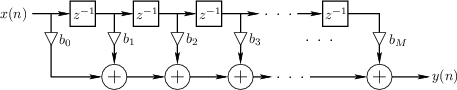
Here we can easily see that the input signal is "tapped" at M+1 places in order to produce the output. The number M is also known as the order of the filter. Without going into detail, the higher the filter order, the closer it can be made to approximate a desired response.

An ideal low-pass filter, which is what we're aiming for, has a perfectly flat frequency response up to the cut-off, above which the input is fully attenuated. This is only possible with an infinitely long sinc filter, so some compromise is necessary. The deviation from the ideal can be described in terms of passband flatness (ripple), stop-band attenuation, and width of the transition band.

Suppose we want to resample CD audio to twice its original rate. We want to minimise ripple below 20 kHz and maximise attenuation above 22 kHz (half the input sample rate). The interval between 20 kHz and 22 kHz, transition band, is unimportant. It is inaudible, and besides, the recording/production process has probably already mangled the content in that range.

First, consider a case with modest requirements, 0.1 dB passband ripple and 80 dB stopband rejection. Plugging these constraints into the Matlab filter designer using the equiripple method, we get a filter of order 147 (that's 148 taps) with this magnitude response:

Zooming in on the passband, we can see that the ripple meets the requirement:

This might be good enough for, say, a portable audio player where cost and power consumption are more important than extreme performance. We are, however, building a high-end system and want something better. Hence, we tighten the specification to 0.0001 dB passband ripple and 180 dB stopband rejection. This produces a filter of order 394, and the magnitude response looks exactly as requested:

This level of performance far exceeds all established limits of audibility. Furthermore, it exceeds the capabilities of any amplifier. This is where any reasonable person would stop and call it good enough. But what if, like Rob Watts, we are not reasonable and believe we can hear things at -300 dB? Matlab can help. The equiripple design method doesn't work with this constraint, so we switch to the window method. Using a cut-off frequency of 21 kHz and suitable window parameters, we get a filter of order 1000 with this response:

Passband ripple is virtually non-existent (note the scale on the y axis):

Given the analogue limitations imposed by physical reality, overkill doesn't begin to describe this. And yet Rob Watts wants to use a filter that is ONE THOUSAND times longer again. It's beyond ludicrous.

It should also be noted that in the M-scaler tests published by Stereophile, it doesn't come anywhere close even to the second filter shown above, so all those taps are essentially wasted.

 

[Veri]

It should also be noted that in the M-scaler tests published by Stereophile, it doesn't come anywhere close even to the second filter shown above, so all those taps are essentially wasted.

Right. To that I can only ask, "how come". Is the premise of Chord's scaler, besides insanely overkill, also a marketing lie? Or is what Stereophile measured basically the target they intended...?

 

[abdo123]

The big issue is that my room has extreme bass dips in frequency at my listening position. It might help, at least Moore than my qutest.

Wouldn’t it be much cheaper to just get 4 subwoofers? 2 below the ceiling 2 on the floor in the middle of each wall instead of fixing the dip for just one person?

 

[Gurra1980]

Wouldn’t it be much cheaper to just get 4 subwoofers? 2 below the ceiling 2 on the floor in the middle of each wall instead of fixing the dip for just one person?

It would be nice, but getting 4 subs and keeping my DAC, don't think I can afford that. My budget is already broken

 

[mansr]

My budget is already broken

Chord DACs tend to have that effect.

 

[Zensō]

Yes that's what I thought, so what you can do I guess is choose one of the five and then shape the curve around it? Is this correct?

Here you go: https://www.rme-audio.de/downloads/adi2dac_e.pdf