
This article is to expand upon earlier discussions about reflections and their potential for harm in a digital transmission system as applied to the audio world. I will be qualitative as much as possible, but numbers are bound to creep in. This is also not meant to be a rigorous analysis, more a hand-waving explanation to help folk see what is happening in their system.
First consider a digital driver (source) and load (receiver) connected by a transmission line (cable). The driver and cable are matched with impedance Zo, and the load has mismatched impedance Zx as shown in the figure below. At the top, a single pulse is launched from the source toward the load. The pulse, now a forward signal, travels down the line to the receiver. Even at nearly the speed of light it takes a little time to get there.
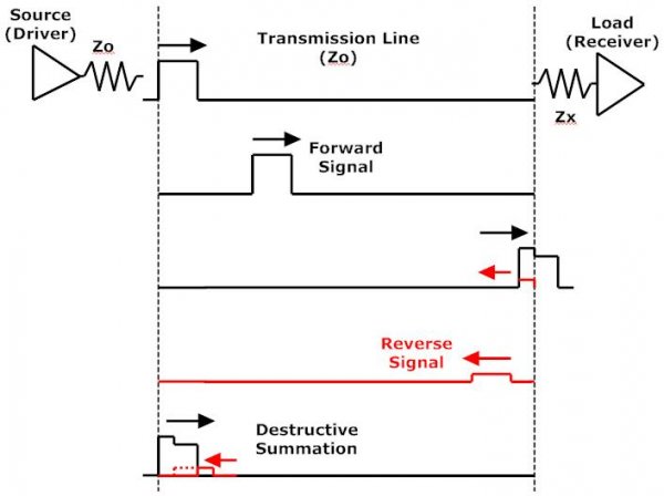
As the signal hits the load, the difference in impedances causes part of it to “bounce back” or reflect from the load. How much depends upon the mismatch; no mismatch, no reverse wave. The reflected signal, which is actually inverted from the original, travels back toward the source (the reverse signal).
In this example, the reverse signal meets the next pulse from the driver near the source end of the line. Where that actually happens depends upon the pulse (bit) rate and length of cable. When the forward and reverse waves meet, some change in the forward signal occurs as the reverse signal interacts with it. In this case, destructive summation is shown, as the out-of-phase reverse signal cancels some of the forward signal pulse. If you hold a hose that has water flowing out of it in your left hand, and try to mate it to a different hose in your right hand, what usually happens is you don’t get perfect alignment and some of the water squirts back on your left hand. Same sort of idea…
Now, Figure 1 shows a periodic pulse train that might be produced by a string of digital data that simply alternates (0,1,0,10,1…) every 250 ns (4 Mb/s). Red is the original signal from the source, blue shows the reflected wave (1/10th amplitude and 180 degrees out of phase), and green shows the resulting pulse train. I have deliberately placed the edges of the reflected wave coincident with the edges of the forward (source) wave.
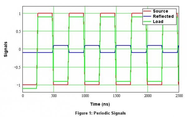
Figure 1. Periodic pulse train.
Now, reducing the amplitude has to change the edge (slew) rate, so this could cause the actual center (zero) crossings to move. That would cause jitter. However, as Figure 2 shows, for an ideal periodic pulse sequence like this, no damage is done. This shows the period measured (histogram) for each of 100 edges. The red box represents the ideal signal and is a single period; the box’s width merely makes it easier to see. The blue stem line represents the signal at the load after reflection. If any period was not exactly 250 ns we would see additional spikes in the histogram. In this case, both ideal and load signals have 100 “hits” at 250 ns, with no errors. As I am tired of making pictures, you’ll have to trust me when I say changing the phase of the reverse wave (moving it with respect to the forward wave) does not matter – a perfect histogram still results.
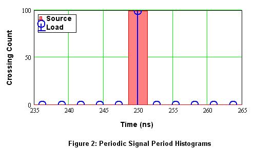
Figure 2. Period histogram of crossings for ideal (red) and load (blue) signals.
While there are many things that can cause variation in even a regular pulse train, let’s move on and consider what happens when the forward and reverse signals are different. After all, a real digital bit stream is not a regular sequence, but varies with the signal. There may be random-length strings of 1’s and 0’s distributed among the signal stream, so in general the signal is not at all regular and periodic like the first example.
Figure 3 shows a reverse signal (blue) three times the length of the source (red). To simplify the simulation, I made it a regular sequence as well, but of course in real life both streams will look essentially random (a function of the signal). In this example, the reverse wave interacts with the bit stream along the cable. We’ll look at the period assuming the bit stream alternates between a stream of single 0/1 transitions (0,1,0,1…) and a 000/111 sequence (0,0,0,1,1,1,0,0,0,1,1,1,…) Notice the output signal (green) is now modulated with the reverse signal. With real data, the forward and reverse signals will in general be different. We again care about what happens at the load, where the two streams interact and the resultant signal is measured by the receiver.
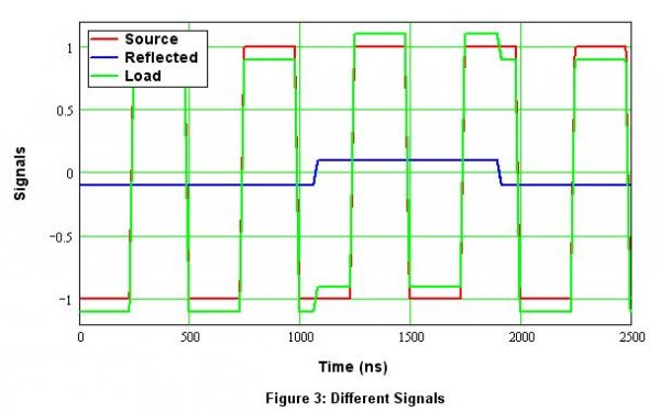
Figure 3. Reverse signal with period 3x the forward signal
Figure 4 shows the resulting histogram. Now, the ideal source still has only one bin centered at 250 ns as expected. However, the load signal is now distributed into three bins, indicating three slightly different periods. This is deterministic jitter – that is, jitter related to the signal (and clock) period, length of cable, amount of mismatch, etc.
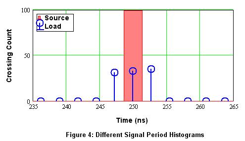
Figure 4. Period histogram with different forward and reverse signals.
So long as the jitter is fairly small, the receiver will have no problem capturing the right data bits. With a 250 ns bit period, no practical receiver would have issues getting the bits right with just a few ns of jitter as shown in this example.
The problem comes when those edges are used to generate the clock for (e.g.) a DAC. The clock circuit will tend to reject small random movements (random jitter), but when patterns like this occur due to a combination of signal bits, clock rate, impedance mismatches, and cable length (among other things), the clock circuit may actually follow the periodic variations and change the clock period accordingly. It has no way of knowing the deterministic jitter is not clock drift, and we get jitter in the output of our DAC. Bummer!
Of course, in the real world there will many different periods and thus many bins of various magnitudes. The jitter threads delve into the magnitude of jitter that might cause problems. In this case, the magnitude is a function of the mismatches among source, load, and cable in the link. Clearly, or perhaps not so clearly, if the cable is the right multiple of the clock frequency (bit period), then any “glitches” will happen at the same time and again no harm done. In general, that is very difficult, as there are a myriad of parameters to control – many of which are in fact beyond our control – and of course the critical length will be different for each data (bit) rate.
Please do not take this as a rigorous proof, but hopefully it helps show some of the things that can go wrong when digital and analog meet, even if we think it’s all digital… - Don
First consider a digital driver (source) and load (receiver) connected by a transmission line (cable). The driver and cable are matched with impedance Zo, and the load has mismatched impedance Zx as shown in the figure below. At the top, a single pulse is launched from the source toward the load. The pulse, now a forward signal, travels down the line to the receiver. Even at nearly the speed of light it takes a little time to get there.
As the signal hits the load, the difference in impedances causes part of it to “bounce back” or reflect from the load. How much depends upon the mismatch; no mismatch, no reverse wave. The reflected signal, which is actually inverted from the original, travels back toward the source (the reverse signal).
In this example, the reverse signal meets the next pulse from the driver near the source end of the line. Where that actually happens depends upon the pulse (bit) rate and length of cable. When the forward and reverse waves meet, some change in the forward signal occurs as the reverse signal interacts with it. In this case, destructive summation is shown, as the out-of-phase reverse signal cancels some of the forward signal pulse. If you hold a hose that has water flowing out of it in your left hand, and try to mate it to a different hose in your right hand, what usually happens is you don’t get perfect alignment and some of the water squirts back on your left hand. Same sort of idea…
Now, Figure 1 shows a periodic pulse train that might be produced by a string of digital data that simply alternates (0,1,0,10,1…) every 250 ns (4 Mb/s). Red is the original signal from the source, blue shows the reflected wave (1/10th amplitude and 180 degrees out of phase), and green shows the resulting pulse train. I have deliberately placed the edges of the reflected wave coincident with the edges of the forward (source) wave.
Figure 1. Periodic pulse train.
Now, reducing the amplitude has to change the edge (slew) rate, so this could cause the actual center (zero) crossings to move. That would cause jitter. However, as Figure 2 shows, for an ideal periodic pulse sequence like this, no damage is done. This shows the period measured (histogram) for each of 100 edges. The red box represents the ideal signal and is a single period; the box’s width merely makes it easier to see. The blue stem line represents the signal at the load after reflection. If any period was not exactly 250 ns we would see additional spikes in the histogram. In this case, both ideal and load signals have 100 “hits” at 250 ns, with no errors. As I am tired of making pictures, you’ll have to trust me when I say changing the phase of the reverse wave (moving it with respect to the forward wave) does not matter – a perfect histogram still results.
Figure 2. Period histogram of crossings for ideal (red) and load (blue) signals.
While there are many things that can cause variation in even a regular pulse train, let’s move on and consider what happens when the forward and reverse signals are different. After all, a real digital bit stream is not a regular sequence, but varies with the signal. There may be random-length strings of 1’s and 0’s distributed among the signal stream, so in general the signal is not at all regular and periodic like the first example.
Figure 3 shows a reverse signal (blue) three times the length of the source (red). To simplify the simulation, I made it a regular sequence as well, but of course in real life both streams will look essentially random (a function of the signal). In this example, the reverse wave interacts with the bit stream along the cable. We’ll look at the period assuming the bit stream alternates between a stream of single 0/1 transitions (0,1,0,1…) and a 000/111 sequence (0,0,0,1,1,1,0,0,0,1,1,1,…) Notice the output signal (green) is now modulated with the reverse signal. With real data, the forward and reverse signals will in general be different. We again care about what happens at the load, where the two streams interact and the resultant signal is measured by the receiver.
Figure 3. Reverse signal with period 3x the forward signal
Figure 4 shows the resulting histogram. Now, the ideal source still has only one bin centered at 250 ns as expected. However, the load signal is now distributed into three bins, indicating three slightly different periods. This is deterministic jitter – that is, jitter related to the signal (and clock) period, length of cable, amount of mismatch, etc.
Figure 4. Period histogram with different forward and reverse signals.
So long as the jitter is fairly small, the receiver will have no problem capturing the right data bits. With a 250 ns bit period, no practical receiver would have issues getting the bits right with just a few ns of jitter as shown in this example.
The problem comes when those edges are used to generate the clock for (e.g.) a DAC. The clock circuit will tend to reject small random movements (random jitter), but when patterns like this occur due to a combination of signal bits, clock rate, impedance mismatches, and cable length (among other things), the clock circuit may actually follow the periodic variations and change the clock period accordingly. It has no way of knowing the deterministic jitter is not clock drift, and we get jitter in the output of our DAC. Bummer!
Of course, in the real world there will many different periods and thus many bins of various magnitudes. The jitter threads delve into the magnitude of jitter that might cause problems. In this case, the magnitude is a function of the mismatches among source, load, and cable in the link. Clearly, or perhaps not so clearly, if the cable is the right multiple of the clock frequency (bit period), then any “glitches” will happen at the same time and again no harm done. In general, that is very difficult, as there are a myriad of parameters to control – many of which are in fact beyond our control – and of course the critical length will be different for each data (bit) rate.
Please do not take this as a rigorous proof, but hopefully it helps show some of the things that can go wrong when digital and analog meet, even if we think it’s all digital… - Don
Last edited by a moderator:
") ) recommends using a 1.5 meter cable to help deal with the reflections. Does that look like a good idea?
) recommends using a 1.5 meter cable to help deal with the reflections. Does that look like a good idea?