Radio Frequency (RF) Analysis of Speaker Cables/Reflections

[Speedskater]

Cat5 cable is 100 Ohm per pair. 4 pairs in 1 cable. so you can make a 25 Ohm cable with one cable and thus need 3 of those cables in parallel.
This will get you close to 8 Ohm with a very low investment.

This is know as the 'Radio Frequency Characteristic Impedance' and it's only true at radio frequencies (that's well above 100kHz).
And even then it's only a well behaved transmission line, if the source, cable and load 'Radio Frequency Characteristic Impedance' are equal.

 

[DonH56]

I probably wrote the original of that post ten-plus years ago before porting it to WBF (and Amir kindly ported it here) in response to a blog about how much transmission line theory and matching impedances mattered for speaker cables. And before that I wrote a similar blurb back in the 1980's. I imagine many other folk have as well. The original intent was to show how silly applying transmission line theory to speaker cables was. Note the rise times are in the microsecond range, way above audio, so any steps are going to be heavily filtered and triple-transit is hardly an issue.

RF transmission line theory does apply, and work, at frequencies well below 100 kHz, however. There are still long-wave (ELF) radios and for that matter the power grid depends on transmission line theory to reduce loss over miles of cable. It all comes down to EM and the old Maxwell's Equations that work down there as well as at microwave frequencies. Maybe better since so many other factors come into play and mW/mmW and up frequencies. There are times I wish I'd gotten a job in audio instead of having to worry about skin effect, dispersion, surface roughness, loss tangents, and all that jazz.

Edit: That is probably a caution for many of these little tutorials. They provide some basic introductory material targeting an audience with at least HS math skills but, while the basic material should still be accurate, the context may be lost in some cases and there are undoubtedly parts that are out of date. For instance, virtually every DAC reclocks and uses circuitry to suppress incoming clock jitter; at the time I wrote some of the jitter articles, that was rare, and in fact some AVRs exhibited 50~100 ns (!) jitter. Unlikely to see that these days.

 

[mansr]

RF transmission line theory does apply, and work, at frequencies well below 100 kHz, however. There are still long-wave (ELF) radios and for that matter the power grid depends on transmission line theory to reduce loss over miles of cable. It all comes down to EM and the old Maxwell's Equations that work down there as well as at microwave frequencies.

Don't forget the good old analogue telephone (or telegraph) line. Not that long ago, you could still find, in rural areas, old phone lines using individual, uninsulated wires strung between poles. The pairs would be rotated a quarter turn for each pole, thus producing a twisted pair line with a pitch around 250 m.

Maxwell's equations, as you say, obviously apply at any frequency. In this context, I think the point is that the resistive losses in any actual cable mean that for low frequencies, the characteristic impedance deviates quite far from the idea which is much better approximated at high frequencies. A 50 Ω coax thus has a rather different characteristic impedance at audio frequencies. Attempting to match the cable impedance to the speaker across the audio range is clearly a fools errand (audiophool's?). Thankfully, there is no need for matching since whatever reflections occur are harmless.

 

[Speedskater]

RF transmission line theory does apply, and work, at frequencies well below 100 kHz,

It sure does, if and only if your cables are miles long!
Two decades ago, Cyril Bateman (RIP) did a serious study of speaker cables as transmission lines. The short answer is, just do a 'RLC' model and be done with it. Even then with the exception of very low impedance (at high frequencies) loudspeakers, a 'R' model is all you need.

 

[wynpalmer]

This is an article our technical member @DonH56 kindly wrote on another forum and place. I am copying it here given the recent interest in its content:

Apples vs. oranges, anybody? In this thread we’ll take a look at speaker cables from an RF perspective, not something usually discussed. Although closer to my professional life than the usual audio analysis, I would not have thought of this except for the prodding by (“interaction with” if you prefer) a fellow engineer. I would have said transmission line effects at audio frequencies are negligible. Was I wrong? Well, the jury is still out, but it makes for an interesting thread, so here we go!

Recall that wires have impedance terms (resistance, inductance, capacitance, conductance – RLCG) distributed along their length. They reduce the cable’s bandwidth, reduce the effective damping factor at the speaker terminals, and add distortion (though the cable’s nonlinearity at audio is insignificant – I am not covering that now). Also remember that it takes time to get from one end of the wire to the other, even for an ideal line. Finally, you may recall from the DAC Reflections thread that mismatches among the source (amplifier), line (speaker cable), and load (speaker) impedances cause reflections. That is, not all the energy goes straight into the load as we would hope, but some gets reflected back. The bigger the mismatch, the bigger the reflection, the less signal is initially delivered to the load, and the longer it takes to settle to its final value.

First, let’s get the equations out of the way:


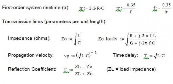
Figure 1: Equation set.

Note vp is for the electrical signal, not the sound waves out of the speaker! Sound travels around 1130 feet/s, while the signal in the wires typically travels about 1/2 the speed of light (1/2 of 186 thousand miles/s) for an audio cable (can be 0.9c or more for RF cables). The good news is I am not going to use these equations any more, but they are the basis of the pictures that follow. For more info, look up transmission lines on Wikipedia or your favorite RF handbook.

Now let’s look at a simple circuit formed by an ideal amplifier (a perfect voltage source), a short (20-foot) speaker cable, and ideal 8-ohm resistor to model the speaker. For speaker cables I used an ideal and lossy 8-ohm cable, and ideal and lossy 93-ohm cable that is essentially the original Monster Cable. The delay time is ~45 ns for these cables. I applied a step input with a 10 ns edge (8 ns rise time, equivalent to ~44 MHz bandwidth). The results for several test cases are shown in Figure 2, with the output voltages measured at the load.



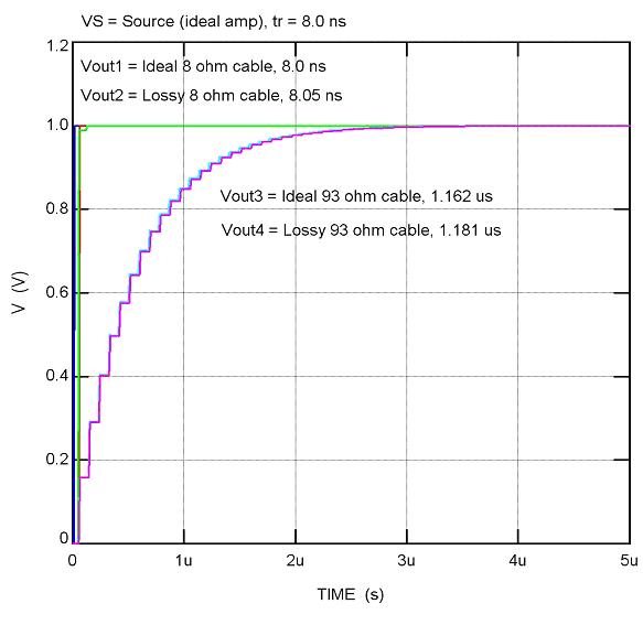
Figure 2: Ideal amp, load trials with 10 ns input step.

Now, with an 8-ohm cable and 8-ohm load the match is perfect so no reflections occur (gamma = 0). It is difficult to see but the ideal 8-ohm cable rises smoothly in 8 ns and starting 45 ns after the input step as expected. The lossy 8-ohm cable is nearly the same, but with one tiny little perturbation at the top (barely visible in the green line) and rise time is 8.05 ns. I cannot imagine anyone would hear any impact from either 8-ohm cable.

The 93-ohm case is much more interesting. Now we see mismatches causing reflections and the resulting longer settling time. Because of the mismatch between line (93 ohms) and load (8 ohms), only part (about 16 %) of the initial energy is absorbed, and the rest is reflected (“bounced”) back to the amp. There it is again reflected (100% since the amp is ideal), and travels back to the load (speaker), adding a bit more power but again reflecting most of the energy back. We see the signal at the speaker building in steps throughout this process. This back and forth goes on for several microseconds as seen in the picture, with the voltage at the speaker gradually rising as a little more energy is passed on to the load at each “bounce”. The effective rise time is now about 1.2 us (~300 kHz bandwidth) – still well above the audible band, but much lower than the ideally-matched case. Again, the difference in rise time between the ideal 93-ohm line (1.16 us) and lossy line (1.18 us) is insignificant.

Let’s talk just a bit about this bouncing that is going on… Some of us are old enough to remember those hard rubber “Superballs”, and the rest have hopefully seen how a small plastic ball bounces. I am going to use that for an analogy (and yes, I know this is not terribly rigorous, please bear with me). The ball is the signal, and the ground the load. What we’d like is for the load (ground) to instantly absorb all of the ball’s (signal) energy, giving nothing back. This would be like throwing the ball into a pool of thick, gooey mud. One splat, and that’s it. The other extreme would be smooth concrete. The ball hits and bounces, bounces nearly as high the second time, and bounces many times before all its energy is gone. Only a little is transferred to the concrete with each contact. In between is something like grass; a few bounces and we’re done. Perfect energy transfer would be like mud, with a reflection coefficient of 0, and concrete is a coefficient of almost 1 with almost no energy transferred.

The question of whether the mismatch matters is an interesting one. I think it is safe to say that a 45 ns reflection is unlikely to be heard by anyone. Our ears should average those little steps so we don’t hear them (I think). As for the effective change in rise time, a 20 kHz sine wave has a rise time of 17.5 us, about an order of magnitude slower than the cable. So, the 93-ohm cable would have to be ten times longer (200 feet) to approach the rise time of a 20 kHz signal. Or, have an impedance ten times higher, i.e. a cable with very low capacitance and/or very high inductance. There may be such cables; I do not know. From a rise time, or bandwidth, perspective the cable does not seem to matter.

The other argument that has been made is how the reflections impact our perception of location. It was shown in a much earlier thread (not one of mine, though I did run some numbers) that we can actually perceive timing changes in the microsecond region. This is based upon our ability to recognize a small shift in location which, when calculated as a time difference between our two ears, works out to just a couple of microseconds. So, might a relative time shift of 1 – 2 us caused by reflections be noticed? The problem with this theory is that, treated as a time constant, again there is an order of magnitude between the cable’s time constant and that of a 20 kHz signal. The audio signal, especially when comprised of many different tones (like music), may well mask the effect. And, the reflections operate upon all signals, meaning all edges are delayed. Finally, if the mismatch is the same for each speaker, the same signal will have the same equivalent time delay for each speaker. Of course, different frequencies will see different impedances in real speakers, thus the reflections will be different for different frequencies. This could cause the image to shift (vary) with frequency. Clearly it can get complicated... What is also clear is that transmission line effects can matter in speaker cables, though whether these effects are audible I can’t say.

One last look at this fairly ideal case: what if a more realistic (slower) rise time is used? A 10 us edge (8 us rise time, a little over 40 kHz) is shown in Figure 3. The reflection “stair steps” are no longer visible and the rise time is essentially the same as the source (8 us) for the 8-ohm and 93-ohm traces. The delay caused by the distributed RLC of the 93-ohm line is visible, however. The 8-ohm lines’ delay is about 45 ns, as expected from T calculated above, but the 93-ohm lines’ delay is about 0.5 us. An ideally-matched line and load renders the LC essentially “invisible”, but a mismatch means the distributed impedance is “visible” and impacts the propagation delay consistent with the effective bandwidth. Again, the audibility is a matter of some debate…



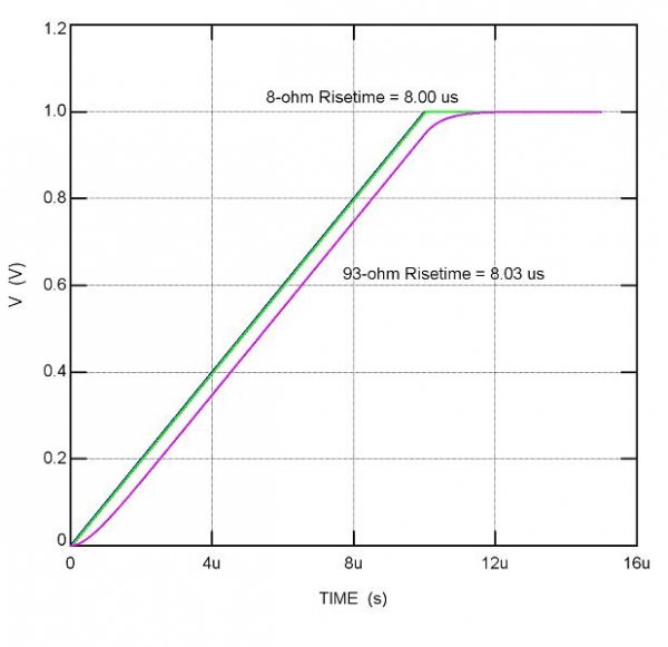
Figure 3: Ideal amp, load trials with 10 us input step.

The analysis for bi-wiring is also very interesting, but another day…

I have a slightly different view on this which some might find valuable.
In any case, here goes.
I modelled the response of a severely miss-matched transmission line, but rather than use the waveform suggested above I used a 1kHz square wave with a single pole RC low pass filter followed by unity gain buffer with a finite source impedance- say 1 ohm. I then used a transmission line of a given delay, in this case 25ns with a (not important) characteristic impedance of 77ohms and a load of 10kohms. The 25ns corresponds to a line with a length of 5m and velocity factor of 0.666....

The low pass was set at a cutoff of 300KHz and the transient and AC responses were plotted.

Above is the AC response. Note that the system actually has substantial resonant gain at 10MHz- or 1/(4x(delay line time)), but does not effect the response at audio frequencies. It does suggest that the power amp needs to have an input band limit applied in order to avoid possible IM issues.
Now for the transient response.

This shows the input waveform, the output waveform and the delta. Note that the delta is an exponentially decaying sinusoid.
This waveform looks identical if the low pass cut off is reduced to say, 100k- but the sinusoid is reduced in amplitude accordingly. A more complex filter that further increases the attenuation at high frequencies further attenuates the sinusoid so that it no longer is visible.
Below is a 3rd order filter with a -3dB point at c. 60kHz.

Anyway, it seems reasonable to view the transmission line action in this case as simply a modification to the frequency response of the system and not invoke any time domain issues at all. This simplifies understanding and allows for mitigation of the effects to be assured.
Essentially ultra wide bandwidth systems are to be avoided unless you want to explore the audible effects of HF generated intermodulation products.

 

[wynpalmer]

It sure does, if and only if your cables are miles long!
Two decades ago, Cyril Bateman (RIP) did a serious study of speaker cables as transmission lines. The short answer is, just do a 'RLC' model and be done with it. Even then with the exception of very low impedance (at high frequencies) loudspeakers, a 'R' model is all you need.

I have a tube amp with hybrid electrostatic speakers so the source and load impedances are quite complex.
I find that a simple RLC model works quite well in predicting measured frequency response for the system.
As is shown in post #25 even if ANY interconnect cable does behave like a transmission line it's still fine to treat it like a lumped network - unless you are foolish enough to have a very wide band system in which case you need to worry about reflection induced resonances.
Basically, have your system be a simple third order LP at 60KHz or so and you're all set- unless you are concerned about the 0.5dB or so "loss" at 20kHz, or the consequent phase shifts and alterations to the system impulse response (I'm not).
IM products generated by power amps due to the presence of supersonic and ultrasonic signals can be quite audible.

 

[DonH56]

The only time T-line theory-like stuff has mattered at audio in recent times for me was the case of an inexpensive class D amplifier (don't recall the brand, it belonged to a friend) that kept blowing fuses driving his MLs. We looked with a 'scope and took a peek at the ML's impedance with a VNA. There was a nasty resonant peak around 1 MHz or so and it interacting with the amp so it broke into full-scale'ish oscillation right around that frequency. The amp's switching frequency put an unlucky spur pretty much right at the resonance peak. We could move it a little using differnt speaker cables but it would not really go away. The load plus amp output filter was enough to attenuate the signal at the output fairly well, but inside the amp it was large and the amp heated up fairly quickly. A little RC snubber was enough to kill it but I also added an integrating cap in the feedback to drop the loop response to provide a bit more margin.

Note in this case, as @wynpalmer showed, the real problem was simply the resonant peak and not t-line theory per se.