I received these questions on the Finnish Hifiharrastajat forum and wanted to share both the questions and my answers here on ASR.
Questions
- Was the original intention to try to determine the direction of just one speaker at a time? Had you then moved on to the “phantom” image created by several speakers working together?
- In the L–C–R case (and other cases where the image/source is placed exactly between two speakers), a phantom image is trivial to produce: there is no need to change phase or level as long as the geometry is precisely symmetrical. Have you made a version that investigates arrangements other than L–C–R, and a sound image or source produced by more than two speakers? Of course, even in the L–C–R case, the speakers’ acoustic centres may differ in height, which seems to show in those plots.
- Have those phantom-image samples also been used to train the recognition network? Or are you aiming for a situation where it would learn to recognise a direction, such as the centre, without having “seen” it? That depends somewhat on what you are trying to achieve. Without phantom examples in the training data, the results could probably be a little difficult even to interpret: the model would naturally try to recognise from the acoustic features whether the right or left speaker is playing, even though both are playing, and the result might oscillate between them. Of course, acoustically, a perfect superposition of the two speakers’ sound waves would appear to come from the centre. I’m mainly wondering whether human ears and brains might be more forgiving of that phantom centre than a neural network that has never seen it.
- And if those samples are included in the training data, that also makes interpretation somewhat difficult: it learns to recognise when two speakers have been played in that particular room and that the direction should be reported as being between them.
My answer
Good questions. The first answer is that there is no neural network involved here anymore. This is a purely calculation-based method, where all the results are obtained from the data by calculating ITD, ILD, phase, GD and other parameters. In that sense, it is a very traditional approach compared with a neural-network-based method. I chose this approach so that the software’s operation can be broken down into its smallest parts more easily, and the calculations could even be reproduced elsewhere. Neural networks are a little too much of a black box in this respect, and I don’t really want to put my trust in that fog.
So the individual answers can be read with that in mind.
1. Originally, I was interested in using a binaural dummy head specifically to determine directions and distances. Later, during a visit, friend suggested measuring stereo imaging, which is what these latest posts have been about. I immediately thought it was a good idea, and it has been really interesting to work on. In my view, this is probably the part with the most interest from a hi-fi perspective.
2. The software can render sound to any speaker or combination of speakers, between speakers, or along a path between speakers in a 7.1.4 system. These can then be measured using the dummy head to check how the system behaves.
Earlier, I posted about a silly bug I found in the software relating to exactly this: it was calculating where the sound landed based on the speakers used for rendering. It was using the speakers as anchors, forcing the sound across the whole frequency range to stay between the relevant speakers, which obviously did not reflect reality. This became particularly clear in the bass when I did the 360° panning measurements. The corrected code allows the sound image to spread wherever it happens to go, so in that respect the calculation better reflects reality.
The challenge here is, of course, the cone of confusion, where the same ITD values can correspond to sound coming from in front or behind. I then came up with my own causal solution to this: with panning, the sound is tracked starting from both/all speakers, and each panning step has a cause-and-effect relationship. This means that if the pan is, say, 10% from L towards R, and the next panning point is 15%, the calculation for 15% follows the ITD, ILD, phase and other data from 10% and the preceding steps, which weight the likelihood of the next value. This still allows the code to get the direction completely wrong, but it is no longer as random as it is without that information.
3. This is a slightly trickier question because, as I mentioned, there is no neural network behind this, so no actual training takes place. However, the calculation does use known references through the solved topology. Once the speakers, room and dummy head have been worked out through blind measurements, the code knows the speakers’ directions and distances. Their data has been stored as a reference, so it knows what each speaker sounds like at the different points where it has been measured.
The phantom data is therefore completely new from the code’s perspective, and there is no direct reference for it. The same ITD, ILD, phase and other quantities are calculated from it as in the other calculations, and those are then used to form the plots showing where the sound falls on the coordinate axes.
The foundation is nevertheless very shaky in the sense that the code has no fixed values to work from. It does not know the size of the dummy head—meaning its acoustic ear spacing—which I think is already a serious challenge to solve in itself. It does not know which direction is up. Nor does it receive an external reference value from which it could calculate TOF, such as a loopback signal. Consequently, its ability to create a speaker map that corresponds to reality is the strongest evidence that the code works. To do that, it has to solve those unknown variables from the supplied measurements with sufficient accuracy.
Ear spacing, for example, is an excellent scale adjustment. When you have a suitably sized head to listen with, everything makes sense to it and all the speakers fall into place at the correct distances.
Those few videos I posted were real ear- and mind-openers for me, because I was already fairly convinced that the code was not identifying the front direction correctly in the L–R measurements. But when I listen to those measurements through headphones, to my ears they correlate with the data very logically. In one, I hear the sound clearly farther away and focused at the centre, whereas the other spreads around my head and partly behind it. In both, I can also hear the direction and distance of the direct L and R speaker measurements really well. This convinces me, at least, that the code is already quite capable of forming a logical graphical representation from the data.
4. As mentioned, because there is no neural network, “learning” is a slightly misleading word. I think it should be called something like “a model formed from measured data,” which better describes the mathematics behind it. But you are certainly right that this is not a general-purpose model that you could simply drop into any room and start measuring sound directions. You can, however, put it into any room and feed it sounds, after which it can establish directions for those sounds with good accuracy.
Below is the mapping data used for these measurements. The measurement points are scattered around the room, and this is the accuracy achieved with them. From experience, I can already say that around seven measurement points give really good accuracy in my setup when measuring all 11 speakers. With a large number of speakers, the constraints between them force the solver’s solution much more strongly than with fewer speakers.
The two-channel map is still far from reality, and I’m convinced that it cannot be solved with this little starting information. There are simply too many free variables in the two-speaker case.
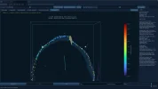
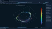
Further down are a few more images of those L–R measurements. They show where the dummy head is positioned relative to the speakers. The dummy head’s position first has to be measured as part of the sound-image measurement process, and only then can the actual sound image be measured.
The images also show clearly how much difference it makes whether the dummy head is near or far away. As I described earlier, when listening from farther away, the phantom sound forms a more point-like image in the centre, whereas up close it spreads all around. The same thing appears in the graphs through the data.
The centre speaker produces an even more focused image in the middle, which is also very clearly audible directly from the measurements. However, the centre speaker is not completely immune to the effects of reflections when the dummy head is very close to the speakers. That also shows in the data and can be heard in the measurements.
Because listening to this is so important, I have added a feature to the software that lets me listen to the measured sounds while seeing, in real time, how the data from that sound forms the graphics.
Now, as I’m adding these pictures, I notice that I need to improve how the code shows which speaker or speakers are playing in each measurement, and perhaps also show their weighting in some way.
Translated from Finnish with AI assistance.