This opening post is to show how to simulate room modes using Mathematica. The other room mode calculators I could find on the web can only handle rectangular box shaped rooms. Mathematica can solve for arbitrarily shaped room. I only attempted 2D, but theoretically Mathematica should be able to compute 3D too. I'll leave that for the ASR high achievers 
Mathematica comes free with Raspberry Pi (Raspbian). I don't have a Pi with me so I haven't tested my notebook on a Pi. This example notebook took several seconds to run on my i7-10750H laptop, with the vast majority of it on generating the plots. I am guessing it wouldn't be too bad on a Pi. I'd love to have some feedback if any of you try it on a Pi. I'd recommend running it on one of the models with larger amounts of RAM.
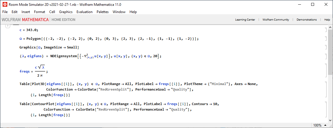
A brief look at the those few (7) lines of code (looks so simple, isn't it ):
):


Mathematica comes free with Raspberry Pi (Raspbian). I don't have a Pi with me so I haven't tested my notebook on a Pi. This example notebook took several seconds to run on my i7-10750H laptop, with the vast majority of it on generating the plots. I am guessing it wouldn't be too bad on a Pi. I'd love to have some feedback if any of you try it on a Pi. I'd recommend running it on one of the models with larger amounts of RAM.
A brief look at the those few (7) lines of code (looks so simple, isn't it
- 'c' is the speed of sound.
- 'Ω' is the domain, which in this case is the room. It is a polygon defined by its vertices. I used 8 vertices in the example. (Rectangular room with 2 corners taken out.)
- Show us the room we are simulating.
- This line does all the computations. It numerically computes the eigenvalues (related to room mode frequencies) and eigenfunctions (room mode shapes). In this example I specified solving for the first 20 modes.
- The returned eigenvalues λ are the square of the acoustic wavenumbers. This line convert them into frequencies in Hz.
- The last two statements are to display the results. The first set of figures shows the mode shape in 3D. The second set shows the contour plots from top so the mode peak locations are easier to see. The reds and greens are locations when the effects of the mode are strong. The white areas are
where it is unaffectedthe nulls.


Attachments
Last edited:


