Understanding How the Klippel NFS Works

[dasdoing]

maybe this can set to lower value ?
here are waterfall with 0.5 0.2 and 0.1 ms. 0.15 ms (as stereophile use)is not possible in REW. but 0.2 ms look good too. I use for all screenshots 100 segments so you can count the segment lines at 7 khz until it reach 65 db. at 0.5 ms rise time i ccount more than 12 segment lines .at 0.2 ms rise time i count 6 segmentlines. at 0.1 ms risetime 5 segment lines. you can see that the decay time look much longer at 0,5 ms rise time.View attachment 120020View attachment 120021View attachment 120019

I see what you mean at 2k-ish.
in the first graph 2k looks prety resonancy, but 0,1ms shows it actualy falls pretty fast

 

[mwmkravchenko]

looking at the waterfall plots I have to ask a simple question. Would the smoothing used in the plots erase any detail when you are using such a short time period? You are basically looking at the bias in the treatment of the original signal used to create the sample and then the mathematics to process this signal. The idea that there is exquisite hidden detail in this type of a plot is not realistic as far as I have seen and worked with.

 

[3ll3d00d]

The rise time in rew is just the width of the left window, i.e. the amount of time included in the analysis before t=0. The waterfall is just that window moved forward x ms at a time. If you make that number v small then naturally high frequencies will rapidly be removed from the window entirely so they will appear to decay quickly just because they have high frequencies and you have cut them out of the window more quickly. If you don't extend the right window by the same amount then there is also some change in frequency resolution because the total length of the window controls this.

 

[bennybbbx]

In Rew manual stand that short rise time giver better time resolution and i think this mean that it show the decay more precise https://www.roomeqwizard.com/help/help_en-GB/html/graph_waterfall.html

The Rise Time control sets the time duration of the Left Hand window. Shorter settings give greater time resolution but make the frequency variation less easy to see. The default setting, 100 ms, is aimed at revealing room resonances. When examining drive unit or cabinet resonances with full range measurements a much shorter rise time would be used, 1.0 ms or lower, with time spans and window settings of around 10 ms. CSD mode may be more useful for such measurements as the later part of the impulse response can be noisy, obscuring the behaviour in the later slices. The 'rise time' terminology dates back to the late 80s and MLSSA. In MLSSA it referred to the 10% to 90% rise time of a left hand window formed by convolving a window function with a unit step (in essence, the step response of the chosen window function). The actual width of the window was much greater, depending on the window type - about twice the rise time for a Hann window, for example, or about 3 times the rise time for Blackmann-Harris. In REW the term is used to refer to the overall width of the left hand window, somewhat misusing it in the interest of retaining terminology that is in common use for CSD plots whilst adopting a definition that provides a clearer indication of what parts of the response lie inside and outside the chosen window settings. To obtain similar results to the MLSSA-style definition use an REW setting that is twice as long.

 

[dasdoing]

In Rew manual stand that short rise time giver better time resolution and i think this mean that it show the decay more precise https://www.roomeqwizard.com/help/help_en-GB/html/graph_waterfall.html

yep, I read that before and came to the same interpretation.

I actualy relooked at my inroom waterfalls again with lower rise time, since the default seams to be for noobs

 

[NTK]

My english is not so good. the time that the waterfall show is 2,94 milliseconds and the waterfall contain 100 segments. each segment(slice) have a line. each line is time 2.94 ms /100 0.0294 ms .with the rise time 0.5 ms there are 4 slices see at near same level at 20 khz. and 4 slices are time 0.0294*4= 0.1176 ms. but 20 khz have a period time of 0.05 ms. so i think when the decay time is so slow as the waterfall show this speaker can not play 20 khz. with rise time of 0.2 or 0.1 sec it look more as reality because when look at the first 4 slices after the impulse the decay time is much more

I suspect some of us may have some confusion or misunderstanding as to how waterfall plots are generated. I would like to describe, as I understood it, how REW generates its waterfall plots and some subtleties of the process. Hopefully, this will help those readers of this thread less familiar with FFT based signal analysis. Apology to @bennybbbx if I am mistaken.

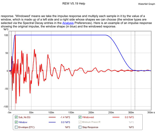
This is from the REW help file. The red curve is the impulse response from a REW measurement, and the blue curve is the "window" used to compute each slice of the waterfall plot. Look closely and you'll see 3 vertical dash lines (I'll call them left, middle, right). The "window" length is the length of time between the left vertical line and the right vertical line. The "rise time" is the length between the left and middle lines.

The window length determines the frequency resolution of each slice (Δf = 1/T, where T is the window length and Δf is the spacing of the frequency bins and therefore, frequency resolution). We cannot determine frequencies at an instantaneous time. There is always a trade-off between time resolution and frequency resolution. We need to know how the signal is changing to measure frequency, and we need multiple samples of the signal spread out in time to do that. The more samples we have, i.e. the longer the sampling duration, the better the frequency resolution but the poorer the time resolution.

Each of the slices in the waterfall plot is the frequency spectrum of the impulse response multiplied with the window. If the window is zero at a certain time location, the signal at that time location is excluded because the product of the window and signal is zero. Therefore, when calculating the frequency spectrum the slice, only the portion of the signal is considered when the window is non-zero.

The slices are generated by moving (sliding) the window to the right in time steps. The time step is the time range of the plot divided by the number of slices (i.e. a time range of 10 ms and 50 slices will give a time step of 0.2 ms). Notice that time step is NOT window length. The duration of the signal used to compute each slice is usually a lot longer than the time step.

The window consists of three regions. There is an initial gradual rise in the shape of the rising half of a raised cosine (half Hann window), a constant horizontal flat line of 1, and a gradual drop at the end in the shape of a falling cosine. The rise time is the length of time of the initial rise from 0 to 1. Therefore, a shorter rise time will give a sharper response to a spike as it moves out of the window quickly as the window slides across the signal.

So why do we need the gradual rise and drop in the window instead of just sharp edges (i.e. a rectangular window)? This is because we want to minimize "spectral leakage". Below is an example using a rectangular window (shaded green). Only the signal inside the green box is used to calculate the frequency spectrum (figure on the right).

However, when we are performing a finite length discrete Fourier transform (as in all FFT), the math actually treats the signal as continuously repeating with a period of the total sampling duration (window time), see below.

If the signal at the start of the window is not exactly the same as at the end, there will be a discontinuity. This type of discontinuity is "spectrally rich", and add spectral contents not present in the original signal. That's why we use smoothly rising and falling windows to smooth out these discontinuities at the start and end of the signal. Therefore, we see a lot of jaggedness in the plots with short "rise times".

Ultimately, the purpose is to evaluate the decay time of the amplitude envelop of an oscillation at the frequency of interest. This decay time number is not very meaningful, and difficult to define, if we are looking at time scales of only a few periods of the oscillation.

 

[bennybbbx]

maybe it is more clear when i show a headphone waterfall at rise time 0.5 and 0.1. see the red arrow. there can see with the 0.5 rise time show near double so long decay time.

the 0.5 rise time show near double so long decay time.

 

[mwmkravchenko]

If the signal at the start of the window is not exactly the same as at the end, there will be a discontinuity. This type of discontinuity is "spectrally rich", and add spectral contents not present in the original signal. That's why we use smoothly rising and falling windows to smooth out these discontinuities at the start and end of the signal. Therefore, we see a lot of jaggedness in the plots with short "rise times".

Ultimately, the purpose is to evaluate the decay time of the amplitude envelop of an oscillation at the frequency of interest. This decay time number is not very meaningful, and difficult to define, if we are looking at time scales of only a few periods of the oscillation.

Exactly. Why it is so important to choose what you look at and how deeply you value and believe it to be true when you are measuring a loudspeaker. So much of what we use to measure is not truly a quantity. Like Air pressure. Or position in time and place in height width and depth phase is the usual term for this type of signal representation. We are looking at derived indications of what is really going on. And if we carefully choose these methods of indicating what is happening either in the time domain, the frequency domain or the spatial 3 dimensions that we live in we can derive some useful information from them. The math gets us short samples and then stitches them together. Most people working with audio measurements gloss over the inadequacy of our means and methods of measurement. This is an interesting an enlightening discussion. Happy to be reading everyones comments. I learn from all of them.

 

[amirm]

the 0.5 rise time show near double so long decay time.

But you shouldn't be looking at these graphs at that level of detail. Only long tails are reliable indications of some resonance. Everything else is so subject to parameters of CSD as to not be useful anyway. This is why I asked you about your request. What insight did you get that was different in one rise time versus another?

Also, unlike how you may be using REW, I set the time window manually, taking care to position the starting one at zero crossing and such. I don't use the auto setting in Klippel software.

 

[amirm]

maybe it is more clear when i show a headphone waterfall at rise time 0.5 and 0.1. see the red arrow. there can see with the 0.5 rise time show near double so long decay time.

Did you go back and compensate by adjusting the impulse window? Of course if you have a slow rise time and leave the start of the window the same, you chop off some of the initial transient.

 

[3ll3d00d]

maybe it is more clear when i show a headphone waterfall at rise time 0.5 and 0.1. see the red arrow. there can see with the 0.5 rise time show near double so long decay time. the 0.5 rise time show near double so long decay time.

if you think through the previous posts about how a window is applied, it will eventually become clear why this is happening. FWIW a v v easy way to see this is a apply a frequency dependent window but get the location of T=0 wrong (i.e. not where the impulse is), your HF content will disappear completely you can also manually recreate the waterfall one slice at a time by shifting the window yourself and comparing the impulse view and the corresponding FR.

 

[bennybbbx]

Did you go back and compensate by adjusting the impulse window? Of course if you have a slow rise time and leave the start of the window the same, you chop off some of the initial transient.

you can see a little on left that acoustic reference is used. but i choose now estimate ir delay. it detect 1,3 samples. that is not much, I see in your latest waterfall that on this B&W https://www.audiosciencereview.com/...kins-607-s2-anniversary-edition-review.21597/ more than 5 slices are near same level. look as this is more than 1.2 ms at 20 khz. and 20 khz have 0.05 ms period.

how many slices do this waterfalls use from you ?.then i can tell you exact how many ms the level at 20 khz does not much decay.

 

[amirm]

how many slices do this waterfalls use from you ?.then i can tell you exact how many ms the level at 20 khz does not much decay.

It is variable because as I mentioned, I adjust it to hit zero crossing. I am not particular as to how many duplicates it shows as long as it is not excessive.

 

[bennybbbx]

know the slice number is usefull to see which time a slice have better. if it is diffrent between measure doesnt matter. only need know how much slices the time range have rew show time range as t=2.94 in my last screenshots. But the slice count not. need look in the gear settings what stand in total slice. maybe show the slice count too is add in future versions

 

[bennybbbx]

here can see the compare of a Monacor RBT-35SR ribbon mid/high tweeter on Kali LP6 and the lp6 own tweeter and the rise time of 0.1 ms show that the ribbon tweeter is much faster with less resonance. with rise time 0.5 is not much diffrence see. i think the banded colour option usefull. on my setting the range is 50 db. this mean every 5 db the color change because 10 colors are possible. the range can also set to 30 db then every 3 db color change.

 

[mwmkravchenko]

here can see the compare of a Monacor RBT-35SR ribbon mid/high tweeter on Kali LP6 and the lp6 own tweeter and the rise time of 0.1 ms show that the ribbon tweeter is much faster with less resonance. with rise time 0.5 is not much diffrence see. i think the banded colour option usefull. on my setting the range is 50 db. this mean every 5 db the color change because 10 colors are possible. the range can also set to 30 db then every 3 db color change.

View attachment 120956View attachment 120957View attachment 120958View attachment 120959

Good application of the waterfall plot.

 

[dkalsi]

Not sure if this question is answered here already, but I was curious if NFS allows one to predict what the speaker may sound like at typical listening distances (e.g. 2.5 meters). I’m just getting into DIY and I’ve read on multiple forms that that response should be optimized for typical listening distance (even if all driver measurements are taken at 1M). When I used various x-over design software (e.g. VituixCAD) - it allows me to design the speaker at various listening distances. When toggling between 1M and 2.5M, there is a difference in the predicted response, albeit minimal.

 

[amirm]

Yes. You can put any number in there. If you just want on axis response it is quick. For the spin data it is buried in the system parameters and is tedious to change. Note that 2m is used but reported at 1m so it is almost what you want.

 

[NTK]

In a nutshell, the NFS is just a tool to obtain free-field (anechoic) measurements without having to have an anechoic chamber. The results from the NFS allow us to predict what the sound field radiated by a loudspeaker at any distances* and directions in 3D space (in the free field/anechoic condition).

The NFS can tell us at what distance far field will begin for the speaker. When I say "far field", I am referring to the term's meaning in acoustics, which is at what distance the loudspeaker begins to behave like a point source (i.e. the listener is far enough away from the loudspeaker that it looks small and integrated). Very often people confuse the terms "near field" with "direct field" and "far field" with "reverberant field". (See http://www.sengpielaudio.com/DirectFieldAndReverberantField.pdf)

The following posts explains how the NFS determines at which distance far field begins.
https://www.audiosciencereview.com/...tudio-monitor-review.15963/page-4#post-513378
https://www.audiosciencereview.com/...tudio-monitor-review.15963/page-4#post-513422



Note: * At any distances further than the measurement locations.

 

[AdamG]

Not sure if this question is answered here already, but I was curious if NFS allows one to predict what the speaker may sound like at typical listening distances (e.g. 2.5 meters). I’m just getting into DIY and I’ve read on multiple forms that that response should be optimized for typical listening distance (even if all driver measurements are taken at 1M). When I used various x-over design software (e.g. VituixCAD) - it allows me to design the speaker at various listening distances. When toggling between 1M and 2.5M, there is a difference in the predicted response, albeit minimal.

Welcome Aboard @dkalsi.