Certainly seems that way - even the 3 way LYD48 doesn't extend particularly low (quoted F6 in "-10hz" mode is 40hz!). But other than that they seem to be surprisingly flat - like maybe +/-1.5-2dB on axis.Just dig up the old review after seeing the latest passive review. As much as I like their look especially the woofer appearance, it seems that in their actives the deepest extension still falls behind the popular Neumann Genelecs and focal?

-
WANTED: Happy members who like to discuss audio and other topics related to our interest. Desire to learn and share knowledge of science required. There are many reviews of audio hardware and expert members to help answer your questions. Click here to have your audio equipment measured for free!
You are using an out of date browser. It may not display this or other websites correctly.
You should upgrade or use an alternative browser.
You should upgrade or use an alternative browser.
Dynaudio LYD 5 Studio Monitor Review
- Thread starter amirm
- Start date
yea, but coupled with their price it does seems the Genelec and Neumann 4" model are more appealing with smaller footprint and more full ranged sound, the on axis response isn't noticeably better for the DynaudiosCertainly seems that way - even the 3 way LYD48 doesn't extend particularly low (quoted F6 in "-10hz" mode is 40hz!). But other than that they seem to be surprisingly flat - like maybe +/-1.5-2dB on axis.
Not sure if you watched Erin’s (@hardisj, just to tag him) talk with Klippel (1hr 23min mark):Before I show you the directivity plots, let me post a new measurement I have not shown before which indicates at what distance the speaker acts as if it is in far field:
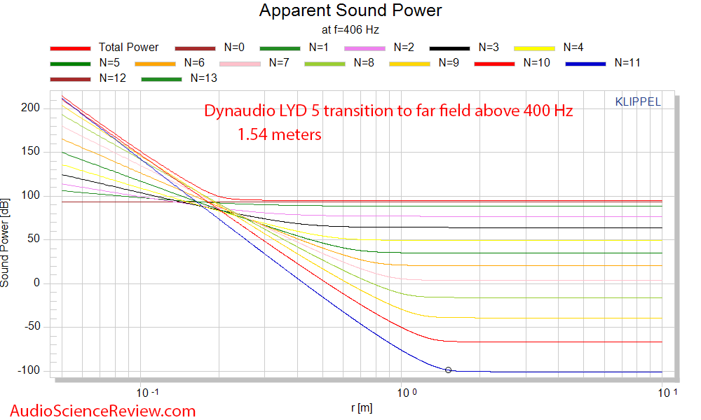
This says that above 400 Hz, that distance is 1.5 meters (where the circles is on blue line) Lower frequencies take forever to get this way so I have excluded them.
You don’t look at the highest order to determine far-field, you look at Total Power. Look at how huge your y-axis is, that is throwing off the intuitive nature, we don’t need the 11th spherical harmonic to be -200dB down from the monopole. He states (as well as one of Klippel’s PDFs) that the far-field limit is when Total Power reaches 0.5dB from being monopole.
Also, showing it at 400Hz just shows it at 400Hz, not it and above. So at 400Hz it’s not 1.54m but around 10^(-0.8)m (your scale is too huge to see 0.5dB increments). This makes sense as it’s mostly the woofer playing that frequency. You stated as you went lower in Hz that the distance increased, which makes sense as this is a rear-ported speaker so the sound field is more complex in the bass and you need to be further away for the port and woofer to sum.
The guy at Klippel said that they are working on generating far-field transition distance for all frequencies, but that it needs work.
However, due to my understanding, there is a manual way. You first look at the Radiated Sound Power graph:
And look at where the monopole nature is most reduced, in this case around 1500Hz.
I am willing to bet if you look at the Apparent Sound Power for ~1500Hz, it will have the max distance to be considered far-field.
_______
Assuming the Apparent Sound Power data can be exported, can it only be exported as 1 frequency (what the graph is limited to), or can you export it for all frequencies? Because if so and you are willing, I can find the far-field distance.
Last edited:
I've had these monitors for a few years and they sounded fantastic. My main issue is the hiss, even on -6db sensitivity. I am sat about 60 cms from the front of the monitors and it is audible, even when music playing. I found that I can still hear the hiss on -6db upto standing 3 metres away. It's really frustrating because I love everything else about them, no other active monitors I find have sounded this good.
I don't think they are faulty because I returned them initially because I was getting static pops when standing up, I received another pair back and they are exactly the same. (I still get the speaking static pops whenever I stand up, which is annoying but I'm half thinking thats a problem with my room/chair/carpet)
I'm just posting this in case anyone had any ideas, or even any suggestions for monitors like these without the hiss - although bear in mind the hiss is the same when nothing is connected to it, so it's not a cable or interface issue either.
Last edited:
Yes, same “issue” for me with these. I suppose maybe I could be super sensitive to noise, but like you, I could hear the hiss from these with nothing playing/no inputs connected from 4 feet away. I’ve read this is due to the internal amplifier that’s being used for these models and there’s nothing that we can do about it. I’ve recently tried the Focal Shape series and I can only hear hiss if I put my ear right up to the tweeter, but it’s silent at my normal listening position. The class AB amps on the Shapes must just exhibit less hiss.I've had these monitors for a few years and they sounded fantastic. My main issue is the hiss, even on -6db sensitivity. I am sat about 60 cms from the front of the monitors and it is audible, even when music playing. I found that I can still hear the hiss on -6db upto standing 3 metres away. It's really frustrating because I love everything else about them, no other active monitors I find have sounded this good.
I don't think they are faulty because I returned them initially because I was getting static pops when standing up, I received another pair back and they are exactly the same. (I still get the speaking static pops whenever I stand up, which is annoying but I'm half thinking thats a problem with my room/chair/carpet)
I'm just posting this in case anyone had any ideas, or even any suggestions for monitors like these without the hiss - although bear in mind the hiss is the same when nothing is connected to it, so it's not a cable or interface issue either.
D
Deleted member 34152
Guest
One of the big differences with the up line (and much more expensive) Core series is better amplification.
The Core series uses Pascal amps. Class D, but with the Core you get heatsinks to match the higher output:
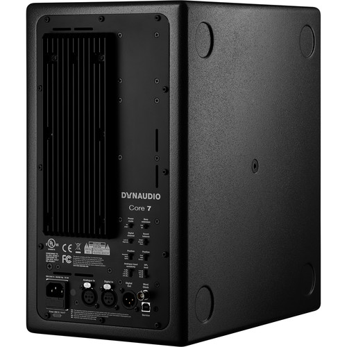
Also has digital input.
FYI, for those interested: I have a pair of Core 47s. The Core 47 is a truly spectacular speaker -- revealing, truthful, and a gorgeous soundstage. But it does have very noticeable hiss in a quiet room (even in a not-so-quiet room if you're sensitive to this kinda thing, like I am) even when nothing is plugged in, and it sucks.
But just to note that the hiss is present even in the much more expensive Cores, just like it is in most other expensive active speakers that I've personally heard, though in varying levels.
Last edited by a moderator:
That's because Amirm is a bass loverI don’t understand how these score so high yet aren’t recommended?

objectively it does well as he said in the conclusion, but that the complete lack of mid to low bass is a huge downside to Amirm and I agree with him, no bass is worse than higher distortion bass, and it's cutoff point is a bit too high for a 5" monitor nowadays
Steve Dallas
Major Contributor
Sounds like the preference rating or recommended is a floored system.
the Kef R3 arguable measures better than revel m16. Besides the kef measuring a touch higher in the treble he calls it “dull”
I just don’t get it
This has been discussed to death on this site and elsewhere.
The preference rating is not endorsed by ASR. It is calculated and supplied by interested members of the site and is considered experimental by many, if not most of us.
Amir has his own preferences for speaker performance, and those who pay attention know he likes bass extension, low distortion, well-controlled directivity, and ability to play loud. YMMV.
The real information is in the spins, and knowing how to read them is key.
yea that's the point, I can live with bad bass extension (if having a sub anyway) and maybe directivity due to very near field listening, review is a review, purchase are based on something more than the basic fact presented and do their own purchase decisionThis has been discussed to death on this site and elsewhere.
The preference rating is not endorsed by ASR. It is calculated and supplied by interested members of the site and is considered experimental by many, if not most of us.
Amir has his own preferences for speaker performance, and those who pay attention know he likes bass extension, low distortion, well-controlled directivity, and ability to play loud. YMMV.
The real information is in the spins, and knowing how to read them is key.
I don’t understand how these score so high yet aren’t recommended?
And the Focal Solo6 with less score and triple the price is recommended...
I understand this is subjective, but it looks too subjective sometimes. Personally, I would remove the boolean recommendation flag and the panther, and for each speaker print the scores and some list of cons and pros.
watchnerd
Grand Contributor
maybe directivity due to very near field listening
This is an important point.
I have the LYD 5 and use them nearfield (<1 m).
I hope anyone who understands their intended use case will understand how to weigh (or not) directivity for any near field monitor.
BoredErica
Addicted to Fun and Learning
It'd be nice to see this test in the future for near-field speakers.Before I show you the directivity plots, let me post a new measurement I have not shown before which indicates at what distance the speaker acts as if it is in far field:
View attachment 82719
This says that above 400 Hz, that distance is 1.5 meters (where the circles is on blue line) Lower frequencies take forever to get this way so I have excluded them. Let me know if you like to see this display for future near-field monitors.
DualTriode
Addicted to Fun and Learning
- Joined
- Oct 24, 2019
- Messages
- 903
- Likes
- 594
It'd be nice to see this test in the future for near-field speakers.
Near Field:
Place small narrow FR speakers on the desk or on stands.
Far Field:
Place larger speakers 2 plus meters away.
What does this test mean and or measure? Is this different that small speakers up close and big speakers farer away?
Thanks DT
BoredErica
Addicted to Fun and Learning
It measures how close you can sit to a speaker and have the drivers sum up correctly. Imagine a giant speaker, x5 size of a regular bookshelf. The distance between the tweeter and woofer is quite large. If I sit close and tweeter is at ear level, that woofer is so far below me and I'm so close to the tweeter that the speaker won't sound right. It seems like the effect in practice in most cases is not super big. However some people like to sit super close and want that peace of mind. 2 way coaxial speakers perform the best in this metric.Near Field:
Place small narrow FR speakers on the desk or on stands.
Far Field:
Place larger speakers 2 plus meters away.
What does this test mean and or measure? Is this different that small speakers up close and big speakers farer away?
Thanks DT
This is why Genelec has specs for recommended listening distance, with the distance increasing as speakers get larger, and decreasing if they are coaxial. Neumann has recommended and minimum listening distance for their speakers.
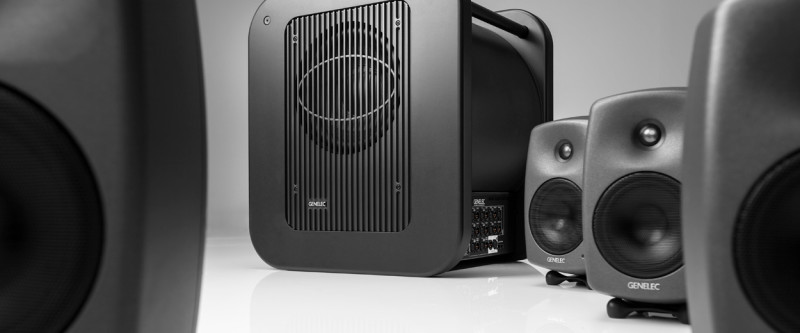
Correct Monitors - Genelec.com
A monitor, by definition, observes, checks, controls, warns or keeps a continuous record of something. An audio monitor, studio monitor or monitoring speaker is more than just a good-sounding loudspeaker. It is a device used in the process of recording, mixing or broadcasting audio in any...
 www.genelec.com
Someone knowledgeable feel free to correct me if it's inaccurate.
Last edited:
DualTriode
Addicted to Fun and Learning
- Joined
- Oct 24, 2019
- Messages
- 903
- Likes
- 594
So what is it that a "directivity plot" measures?
Oops, meant to ask what is it that a "Apparent Sound Power" plot measures?
Oops, meant to ask what is it that a "Apparent Sound Power" plot measures?
Last edited:
On axis vs off axis behavior, more or less.So what is it that a "directivity plot" measures?
DualTriode
Addicted to Fun and Learning
- Joined
- Oct 24, 2019
- Messages
- 903
- Likes
- 594
How is the "Apparent Sound Power" measurement made?
Perhaps that will help.
Perhaps that will help.
Last edited:
Similar threads
- Replies
- 19
- Views
- 2K
- Poll
- Replies
- 237
- Views
- 40K
D
- Replies
- 1
- Views
- 325
- Replies
- 341
- Views
- 57K